The simulated annealing algorithm of GMSE
GMSE: an R package for generalised management strategy evaluation
Brad Duthie¹ ², Gabriela Ochoa¹
[1] Biological and Environmental Sciences, University of Stirling, Stirling, UK [2] alexander.duthie@stir.ac.uk
Source:vignettes/SI9.Rmd
SI9.RmdOverview of simulated annealing
The primary algorithm used in GMSE to model manager and user decision-making is the genetic algorithm. As of version 1.0, GMSE also allows for the use of a simulated annealing algorithm (Kirkpatrick, Gelatt Jr, and Vecchi 1983; Černý 1985; Rutenbar 1989). Simulated annealing searches a space of potential solutions (in GMSE, decisions made by agents to maximise their own utility) in an iterative way. Unlike the genetic algorithm, it is not a population focused approach. The simulated annealing algorithm of GMSE instead iterates from an initial \(k = 0\) to a maximum \(k_{max}\). For each iteration, a single solution exists (agent decision; i.e. either a set of user actions or manager policy choices, depending on the agent), then a new potential solution is considered. Under some conditions, the new solution is adopted and the old discarded.
More specifically, the simulated annealing algorithm of GMSE first
initialises a fixed set of potential agent decisions (size
ga_popsize, 100 by default). These potential decisions are
randomly initialised within the search space of possible decisions using
the same function as in the genetic algorithm. The
fitness of each decision is then checked, and the highest fitness
decision initialised is selected to be the initial random agent decision
at \(k = 0\) (this initial seeding of a
population of ga_popsize has been found to greatly improve
performance).
In each iteration from \(k = 0\) to \(k_{max}\), the agent decision is first checked to ensure that it is not over the agent’s budget using the same cost constraint procedure as in the genetic algorithm. If over budget, then an actions are randomly removed until the decision is again within budget. Next, the fitness of the current agent decision is assessed (again using the same fitness function as in the genetic algorithm).
After checking the fitness of the current agent decision, the mutation function of the genetic algorithm is used to explore a new potential agent decision. The potential agent decision is checked and constrained to be within budget if necessary, then the fitness of the potential agent decision is compared with the fitness of the current agent decision. If the fitness of the potential agent decision is higher, then it replaces the current agent decision. If the fitness of the current agent decision is higher, then the potential agent decision replaces it with a probability of,
\[\Pr(replace) = exp\left(\frac{- \left(W_{current} - W_{potential} \right)}{1 - \frac{(1 + k)}{ k_{max}}}\right).\]
In the above, \(W_{current}\) is the fitness of the current strategy, and \(W_{potential}\) is the fitness of the potential strategy. Note that as \(k \to k_{max}\), the probability of the potential strategy replacing the current strategy decreases when the latter has higher fitness.
Overall, the simulated annealing approach has the potential to be faster than the genetic algorithm approach because it does not require a full population of evolving agent decisions. Below, we show how to use the simulated annealing algorithm in place of the genetic algorithm for users and managers, then we compare the performance of the two approaches.
Example use of simulated annealing
Here we use the same example of resource management as was used in
the main introduction to the GMSE package. This
example considers a population of waterfowl that feed off of farmland,
causing conservation conflict with farmers (e.g.,
Fox and Madsen 2017; Mason et al. 2017; Tulloch, Nicol, and
Bunnefeld 2017), while managers attempt to maintain waterfowl
density at a target level. To replicate the example from the main introduction using simulated annealing, we can
set arguments in the gmse function (or
gmse_apply) for user_annealing and
mana_annealing (TRUE or FALSE
whether simulated annealing is used in place of the genetic algorithm
for users and managers, respectively). An additional parameter
kmax_annealing sets the value for \(k_{max}\). Additional relevant parameters
(e.g., mutation rate) are set using the same arguments as used in the
genetic algorithm; below we set mu_magnitude = 1000 to be
aggressive in exploring new areas of parameter space (note the default
mu_magnitude = 10). The code below runs the example using
simulated annealing for agent decision-making.
sim <- gmse(land_ownership = TRUE, stakeholders = 5, observe_type = 0,
            res_death_K = 2000, manage_target = 1000, RESOURCE_ini = 1000,
            user_budget = 1000, manager_budget = 1000, res_consume = 1,
            scaring = TRUE, plotting = FALSE, user_annealing = TRUE,
            mana_annealing = TRUE, kmax_annealing = 100, mu_magnitude = 1000);
## [1] "Initialising simulations ... "
## [1] "Generation 22 of 40"All other gmse parameters are set to default values.
Figure 1 shows the output, which can be compared with the same output from using the genetic algorithm.
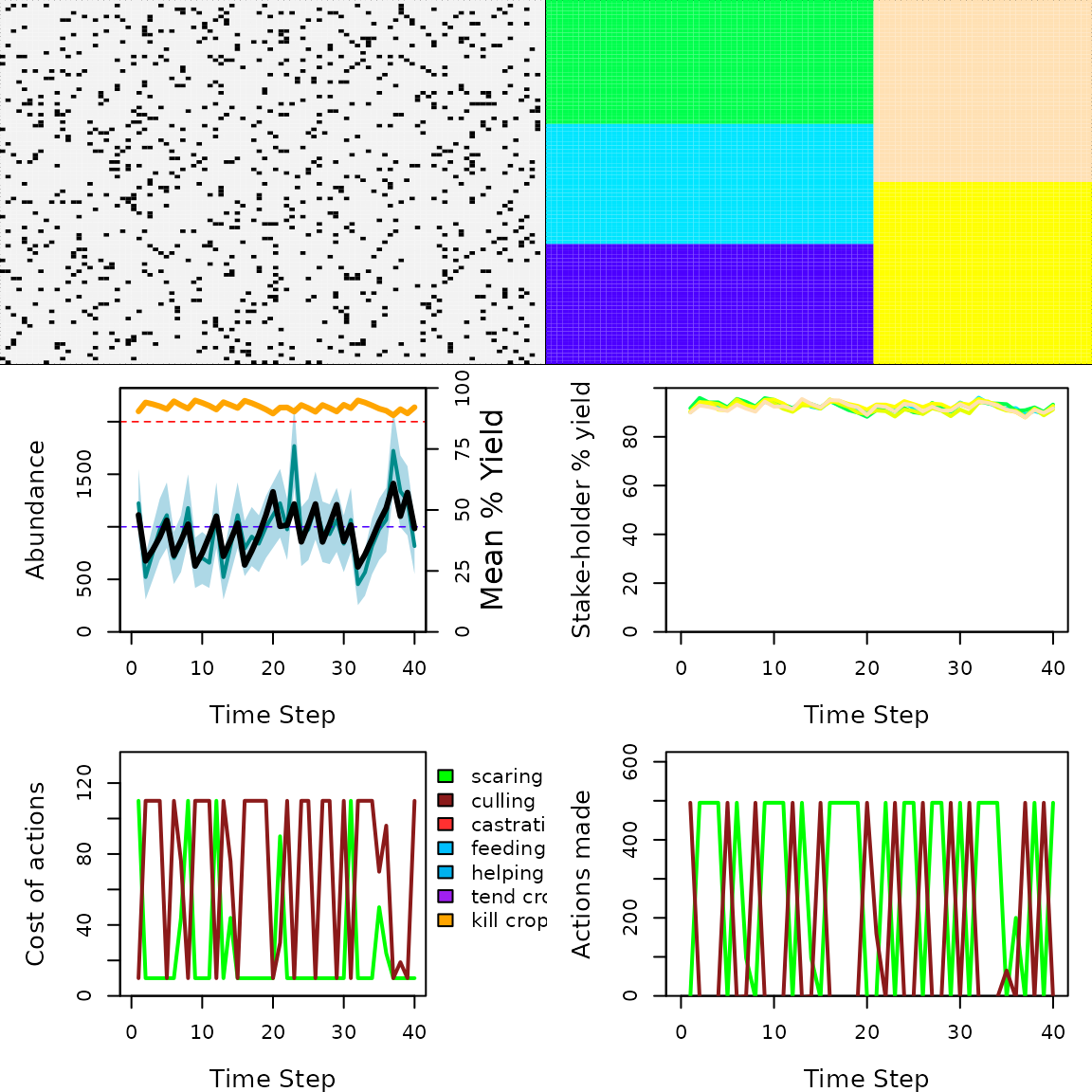
Example GMSE simulation in which a natural resource is managed on the land of five farmers. The upper left panel shows locations of the resource (black dots) on the landscape. The upper right panel shows each farmers land (different colours). The middle left panel shows the abundance of the resource (black line) and its estimate from the perspective of the manager (blue line with 95 per cent confidence itnervals). The middle right planel shows farmer agricultural yield by colour. The lower left panel shows manager policy (costs of farmer actions) over time, and the lower right panel shows farmer actions chosen over time.
Note that the output is the same as is produced the the genetic
algorithm, and any combination of simulated annealing and the genetic
algorithm can be used between managers and users with the
user_annealing and mana_annealing arguments
(but all users must use the same algorithm for decision-making).
Overall, simulated annealing can give faster simulation results, and
often performs better than the genetic algorithm, except when
decision-making is complex for managers. Details of the performance are
described in the next section.
Performance of simulated annealing
Here we show the results of some simulations to compare the performance of the GMSE genetic algorithm and simulated annealing algorithm. The purpose here is to provide some guidance as to when the simulated annealing algorithm might be preferred. The best choice will likely be a trade-off between simulation time and the decision-making ability of GMSE agents. And because agents are, by design, not intended to be perfectly rational, what constitutes desirable ‘decision-making ability’ might also vary with simulation objectives. In other words, there might be situations in which it is desirable for agents to make decisions that are very closely aligned with their goals, and other situations in which it might desirable to have agents make fast but sub-optimal decisions.
Performance in terms of real computation time
First, we show the results of test runs from a highly simplified example in which a single user is modelled (i.e., a lone farmer). In these test runs, the resource, observation, and manager model are simplified to run as quickly possible using the alternative functions introduced for demonstrating the gmse_apply function.
# Alternative resource sub-model
alt_res <- function(X, K = 2000, rate = 1){
    X_1 <- X + rate*X*(1 - X/K);
    return(X_1);
}
# Alternative observation sub-model
alt_obs <- function(resource_vector){
    X_obs <- resource_vector - 0.1 * resource_vector;
    return(X_obs);
}

# Alternative manager sub-model
alt_man <- function(observation_vector){
    policy <- observation_vector - 1000;
    if(policy < 0){
        policy <- 0;
    }
    return(policy);
}
The default user sub-model is then used with a single stakeholder.
sim_old   <- gmse_apply(res_mod = alt_res, obs_mod = alt_obs, man_mod =
                        alt_man, get_res = "Full", stakeholders = 1,
                        X = 10000, ga_seedrep = 0, ga_mingen = ga_min,
                        user_annealing = FALSE, mana_annealing = FALSE,
                        kmax_annealing = kmx, user_budget = 10000);
The gmse_apply function is then looped for 40 time steps
across different values of ga_min (number of generations
for the genetic algorithm) and kmx (number of iterations
for simulated annealing). Higher ga_min and
kmx result in longer computation times, but also
potentially better user decision-making (code is available in the
appendix below). For simulated annealing, we set
mu_magnitude = 1000, but left it at the default
mu_magnitude = 10 for the genetic algorithm. The
decision-making scenario is highly simplified; resources are initialised
to be super-abundant and managed to maintain this abundance (i.e., there
are a lot of resources and managers consistently try to keep it that
way). The best decision for the user is therefore clear. The user should
simply apply their budget to culling as much as possible. Hence, the
number of resources that the user culls can be used as a metric of
decision-making performance. We can therefore investigate the trade-off
between computation time and performance in for the genetic algorithm
and simulated annealing. The results show simulations from a PC running
Xubuntu 18.04 LTS with a Intel(R) Xeon(R) W-2295 CPU (3.00 GHz)
processor, 18 dual threaded cores, and 32 GB RAM.
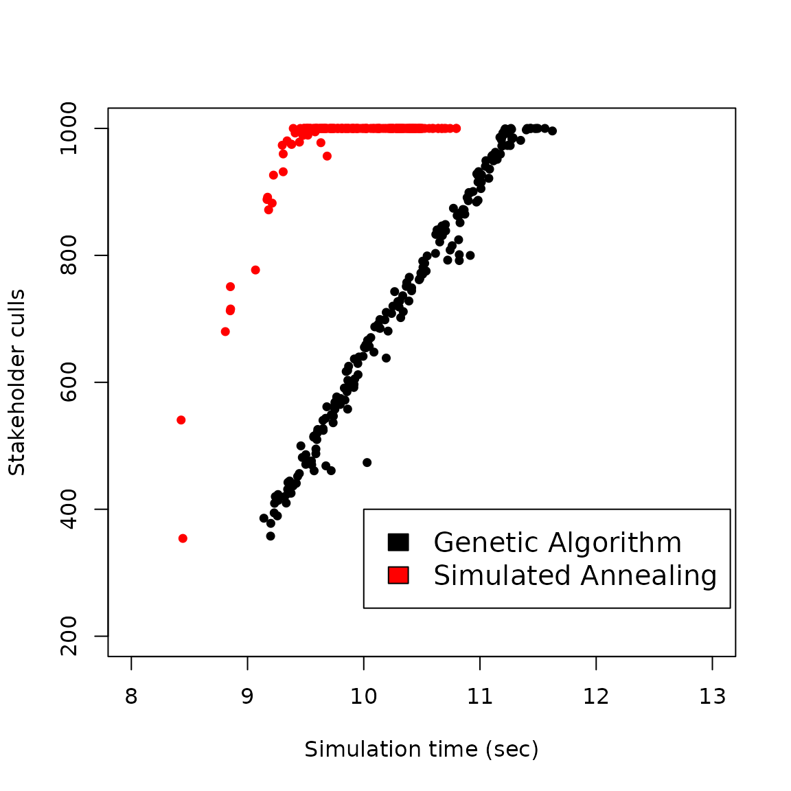
Comparison of stakeholder culls (a metric of decision-making performance) across different simulation times when running a genetic algorithm versus a simulated annealing algorithm in GMSE. Each point represents a unique simulation of 40 time steps run at a specific number of genetic algorithm generations (ga_min) or simulated annealing iterations (kmx).
Results from Figure 2 show that given sufficient time, agents will decide to use all of their actions to cull the highest possible number of resources (1000). But the simulated annealing algorithm finds this solution in less time than the genetic algorithm, suggesting that it can be an effective tool when simulation time is limited (especially if many users need to be modelled within simulations).
The situation of only culling is highly simplified. Users clearly benefit from each additional cull, with no other option to maximise their utility. Note that while this case of decision-making performance is straightforward, performance cannot be as easily measured when multiple actions are available to the user; nor can it be measured easily for the manager. As a proxy for quality of decision-making, we use the fitness measurement produced by the fitness function in the genetic algorithm. That is, we assume that decisions assessed to have higher fitness in GMSE will also be better decisions overall.
User fitness increase fitness function call
We can compare the two algorithms in a slightly different way by
looking at their ‘fitness’ in terms of utility within GMSE. This fitness
is explained in detail in the overview of the genetic
algorithm. Since fitness is calculated the same way in both
algorithms, we can compare how fitness increases in genetic algorithm
generations versus how it increases with iterations of the simulated
annealing algorithm (keeping in mind that generation and iteration times
will vary in practice given other parameters specified in GMSE). For
this, we now use the gmse function parameterised as
below.
sim <- gmse(land_ownership = TRUE, kmax_annealing = 2000, ga_popsize = 100,
            user_annealing = FALSE, mana_annealing = FALSE, ga_seedrep = 0,
            plotting = FALSE, scaring = FALSE, culling = TRUE,
            castration = FALSE, feeding = FALSE, help_offspring = FALSE,
            tend_crops = FALSE, kill_crops = FALSE, mu_magnitude = 10);
Note that land ownership has been turned on, but only culling is
available (e.g., as modelling farmers attempting to cull waterfowl
before they damage their agricultural yield). For simulations with
simulated annealing, we instead set user_annealing = TRUE
and mana_annealing = TRUE in the code above, and set
mu_magnitude = 1000. Instead of recording an agent’s
decision after it has been made, we will now look at how each generation
(genetic algorithm) or iteration (simulated annealing) increases user or
manager fitness (see below) on average. Figure 3 shows how user fitness
increases on average as the number of generations in the genetic
algorithm or iterations of the simulated annealing algorithm increases
(note that there are 5 users in these simulations, but Figure 3 only
looks at the actions of a single user).
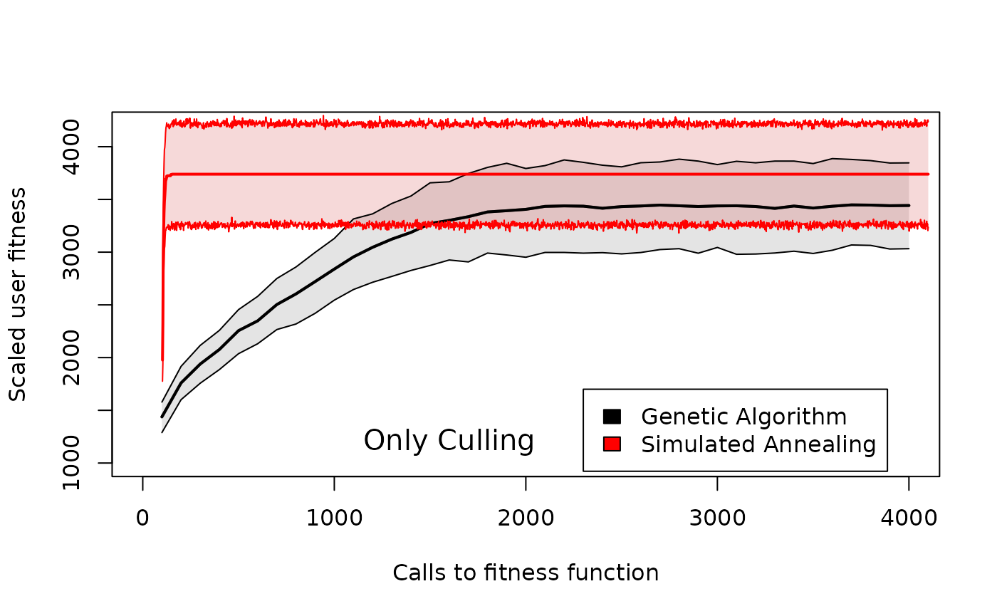
Comparison of user fitness across different genetic algorithm generation numbers or simulated annealing iteration numbers in GMSE when users only have culling available as an action. Shaded areas around the means for the genetic algorithm (black) and simulated annealing (read) show 95% confidence intervals over 100 replicate simulations with identical starting conditions.
From Figure 3, we can see that expected user fitness increases for each algorithm, but the simulated annealing algorithm requires fewer calls to the fitness function than the genetic algorithm to maximise user fitness. Further, the mean scaled user fitness asymptotes to a higher value for the simulated annealing algorithm (unscaled fitness values are much larger, and since the units of these values are arbitrary, we scale them by subtracting the same constant).
This is still, however, a highly simplified case in which culling is the only action available to users. We can compare this with the opposite extreme, in which all seven possible actions are available to users to maximise their fitness. Figure 4 shows fitness increases for each algorithm under these more complex conditions.
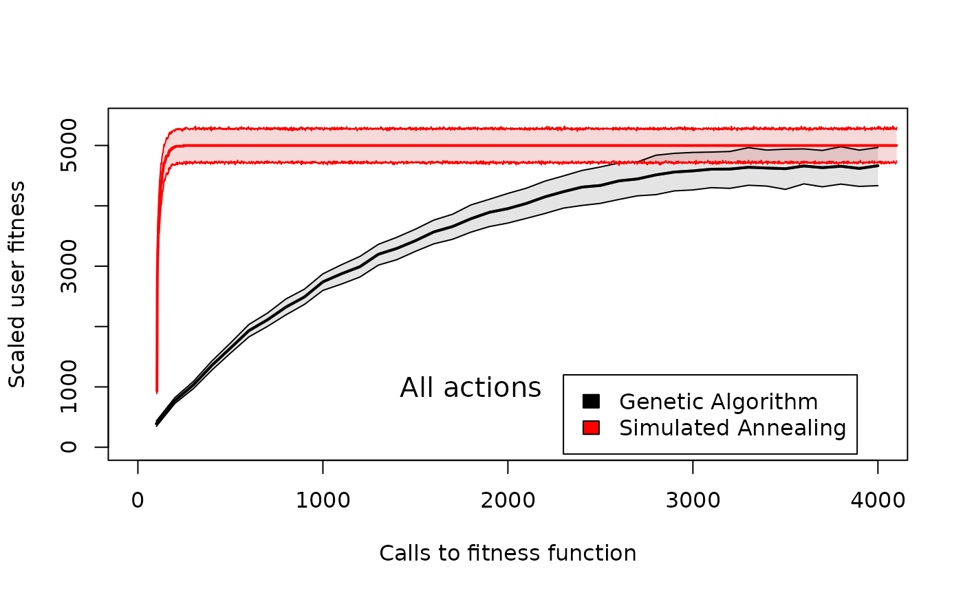
Comparison of user fitness across different genetic algorithm generation numbers or simulated annealing iteration numbers in GMSE when users have all actions available to them. Shaded areas around the means for the genetic algorithm (black) and simulated annealing (read) show 95% confidence intervals over 100 replicate simulations with identical starting conditions.
Under the more complex conditions in which all actions are possible, the simulated annealing algorithm again performs better by finding a higher fitness solution more quickly than the genetic algorithm. Hence, for modelling the decision-making of user agents in GMSE, the simulated annealing algorithm might often be preferred.
Manager fitness increase by iteration or generation
We can now look at the same scenarios of only culling versus all actions from the perspective of the manager. Figure 5 shows the fitness increase for each algorithm when the manager is attempting to maintain natural resources at a target level and culling is the only policy option that they have to use.
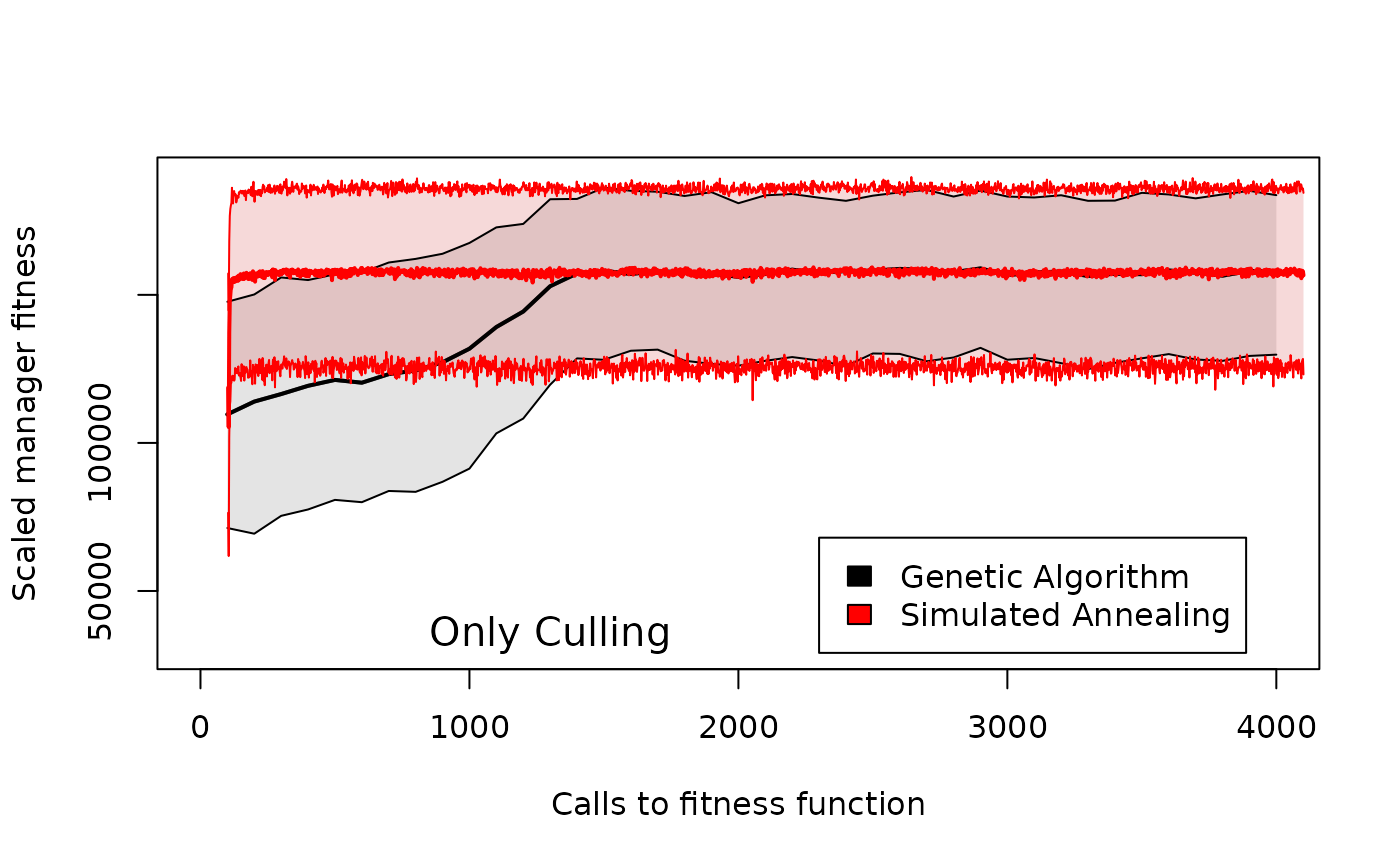
Comparison of manager fitness across different genetic algorithm generation numbers or simulated annealing iteration numbers in GMSE when managers only have culling available as a policy option. Shaded areas around the means for the genetic algorithm (black) and simulated annealing (read) show 95% confidence intervals over 100 replicate simulations with identical starting conditions.
Figure 5 shows that both algorithms appear to be equally capable of finding a solution that maximises manager fitness. But the simulated annealing algorithm finds the solution with fewer calls to the fitness function. The genetic algorithm requires about 15 generations to find the solution (the fitness function is called 100 times in each generation), while the simulated annealing algorithm finds the solution around \(k_{max} = 100\). For simple management decision-making, the simulated annealing algorithm therefore appears to perform at least as well as the genetic algorithm and requires less computation.
The performance of the simulated annealing algorithm versus the genetic algorithm differs, however, when managers have all policy options at their disposal (Figure 6). Under these conditions, the genetic algorithm consistently finds decisions that have higher fitness than the simulated annealing algorithm.
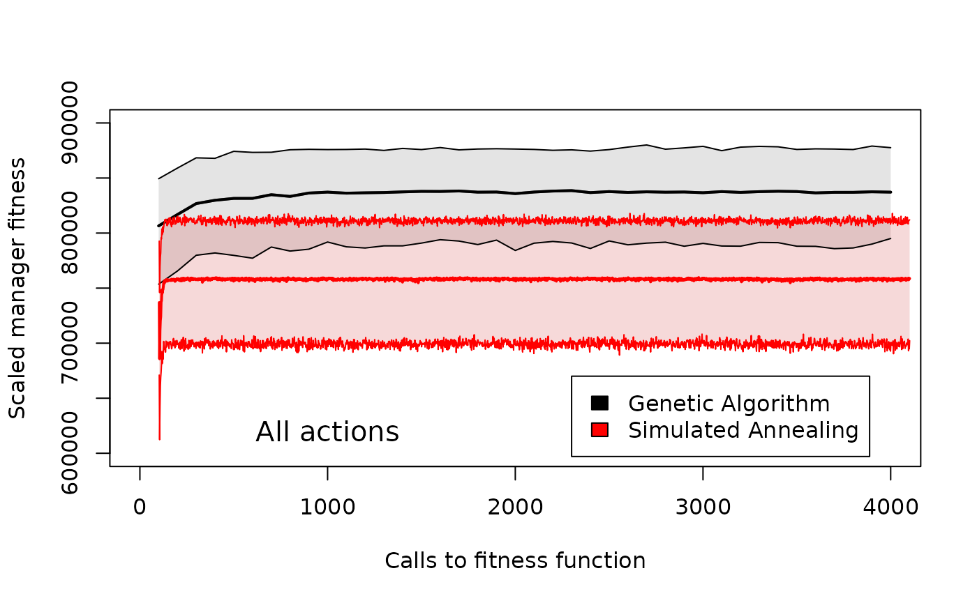
Comparison of manager fitness across different genetic algorithm generation numbers or simulated annealing iteration numbers in GMSE when managers have all policy options available to them. Shaded areas around the means for the genetic algorithm (black) and simulated annealing (read) show 95% confidence intervals over 100 replicate simulations with identical starting conditions.
Given the highly complex situation in which managers must choose from a range of policy options, the genetic algorithm appears to perform more strongly in terms of maximising the utility of the manager.
Conclusion
Simulated annealing can be useful for modelling simple user decision-making. For user agents, the simulated annealing algorithm is likely to be preferable to the genetic algorithm, at least for the current version of GMSE. For manager agents, the simulated annealing algorithm should be used more cautiously, and only when the number of potential policy options that the manager needs to consider is low. Future versions of GMSE might include more complex decision-making for both user and manager agents, potentially limiting the usefulness of simulated annealing. For GMSE v1.0, however, simulated annealing can be highly effective for reducing simulation time and even improving agent decision-making performance.
Appendix code
The code below runs a comparison of the simulated annealing algorithm and genetic algorithm used in Figure 2.
count      <- 1;
AN_summary <- NULL;
GA_summary <- NULL;
while(count < 200){
  time_steps <- 40;
  ga_min     <- 1 * count;
  kmx        <- 1 * count;
  ##############################################################################
  # Genetic algorithm
  ##############################################################################
  st_time   <- Sys.time();
  gal_count <- 0;
  ann_count <- 0;
  sim_old   <- gmse_apply(res_mod = alt_res, obs_mod = alt_obs, man_mod =
                          alt_man, get_res = "Full", stakeholders = 1,
                          X = 10000, ga_seedrep = 0, ga_mingen = ga_min,
                          user_annealing = FALSE, mana_annealing = FALSE,
                          kmax_annealing = kmx, user_budget = 10000);
  gal_count <- gal_count + sim_old$PARAS[[141]];
  ann_count <- ann_count + sim_old$PARAS[[142]];
  sim_sum_1 <- matrix(data = NA, nrow = time_steps, ncol = 9);
  for(time_step in 1:time_steps){
      sim_new                 <- gmse_apply(get_res = "Full",
                                            old_list = sim_old,
                                            res_mod = alt_res,
                                            obs_mod = alt_obs,
                                            man_mod = alt_man);
      sim_sum_1[time_step, 1] <- time_step;
      sim_sum_1[time_step, 2] <- sim_new$basic_output$resource_results[1];
      sim_sum_1[time_step, 3] <- sim_new$basic_output$observation_results[1];
      sim_sum_1[time_step, 4] <- sim_new$basic_output$manager_results[3];
      sim_sum_1[time_step, 5] <- sum(sim_new$basic_output$user_results[,3]);
      sim_sum_1[time_step, 6] <- sim_old$PARAS[[141]];
      sim_sum_1[time_step, 7] <- sim_old$PARAS[[142]];
      sim_sum_1[time_step, 8] <- sim_new$COST[1,9,2];
      sim_sum_1[time_step, 9] <- sim_new$user_budget;
      gal_count               <- gal_count + sim_old$PARAS[[141]];
      ann_count               <- ann_count + sim_old$PARAS[[142]];
  }
  colnames(sim_sum_1) <- c("Time", "Pop_size", "Pop_est", "Cull_cost",
                           "Cull_count", "GA_count", "AN_count", "Cull_cost",
                           "User_budget");

  end_time <- Sys.time();
  tot_time <- end_time - st_time;
  gal_fcal <- sum(sim_sum_1[,6]);
  GA_stats <- c(time_steps, tot_time, gal_fcal, mean(sim_sum_1[31:40,5]));
  ##############################################################################

  ##############################################################################
  # Simulated Annealing
  ##############################################################################
  st_time   <- Sys.time();
  gal_count <- 0;
  ann_count <- 0;
  sim_old   <- gmse_apply(res_mod = alt_res, obs_mod = alt_obs,
                          man_mod = alt_man, get_res = "Full", stakeholders = 1,
                          X = 10000, ga_seedrep = 0, ga_mingen = ga_min,
                          mu_magnitude = 1000, user_annealing = TRUE,
                          mana_annealing = FALSE, kmax_annealing = kmx,
                          user_budget = 10000);
  gal_count <- gal_count + sim_old$PARAS[[141]];
  ann_count <- ann_count + sim_old$PARAS[[142]];
  sim_sum_2 <- matrix(data = NA, nrow = time_steps, ncol = 9);
  for(time_step in 1:time_steps){
      sim_new                 <- gmse_apply(get_res = "Full",
                                            old_list = sim_old,
                                            res_mod = alt_res,
                                            obs_mod = alt_obs,
                                            man_mod = alt_man);
      sim_sum_2[time_step, 1] <- time_step;
      sim_sum_2[time_step, 2] <- sim_new$basic_output$resource_results[1];
      sim_sum_2[time_step, 3] <- sim_new$basic_output$observation_results[1];
      sim_sum_2[time_step, 4] <- sim_new$basic_output$manager_results[3];
      sim_sum_2[time_step, 5] <- sum(sim_new$basic_output$user_results[,3]);
      sim_sum_2[time_step, 6] <- sim_old$PARAS[[141]];
      sim_sum_2[time_step, 7] <- sim_old$PARAS[[142]];
      sim_sum_2[time_step, 8] <- sim_new$COST[1,9,2];
      sim_sum_2[time_step, 9] <- sim_new$user_budget;
      gal_count               <- gal_count + sim_old$PARAS[[141]];
      ann_count               <- ann_count + sim_old$PARAS[[142]];
  }
  colnames(sim_sum_2) <- c("Time", "Pop_size", "Pop_est", "Cull_cost",
                           "Cull_count", "GA_count", "AN_count", "Cull_cost",
                           "User_budget");
  end_time <- Sys.time();
  tot_time <- end_time - st_time;
  ann_fcal <- sum(sim_sum_2[,7]);
  AN_stats <- c(time_steps, tot_time, ann_fcal, mean(sim_sum_2[31:40,5]));
  ##############################################################################
  AN_summary <- rbind(AN_summary, AN_stats);
  GA_summary <- rbind(GA_summary, GA_stats);
  count <- count + 1;
  print(count);
}