Example case study in GMSE

GMSE: an R package for generalised management strategy evaluation (Supporting Information 3)

A. Bradley Duthie¹³, Jeremy J. Cusack¹, Isabel L. Jones¹, Jeroen Minderman¹,
Erlend B. Nilsen², Rocío A. Pozo¹, O. Sarobidy Rakotonarivo¹,
Bram Van Moorter², and Nils Bunnefeld¹

[1] Biological and Environmental Sciences, University of Stirling, Stirling, UK [2] Norwegian Institute for Nature Research, Trondheim, Norway [3] alexander.duthie@stir.ac.uk

An example of management conflict using GMSE

Agents in GMSE (managers and users) are goal-oriented, and their behaviour is therefore driven to maximise a particular utility of interest such as a target density of resources. For managers and users, this could include animals or trees of conservation interest. For users, it could additionally include a landscape harvest size such as bag size or timber. This model feature allows GMSE to evaluate the actions of agents in the context of their individual objectives, and to therefore quantify the degree to which those objectives are or are not achieved. When the actions of one party clashes with the objectives of another party, the objectives of one might be expressed at the expense of the other, causing conservation conflict (Redpath et al. 2013). Currently, there is no standard way to measure conservation conflict in a social-ecological system where both the natural resource (e.g., animals, plants, or non-biological resources) and the people (e.g., stakeholders, managers, etc.) are modelled in a single system, and previous modelling approaches have not meaningfully separated agent objectives from agent actions. We suggest that a starting point to developing a useful metric of conservation conflict is to quantify the deviation of an individual’s actions from their objectives (i.e., of actual actions from desired actions), the former of which is restricted by the actions of other individuals. Here we show how GMSE can be used to evaluate the amount of conflict in a simulated social-ecological system under different management options.

To demonstrate how GMSE can be used to understand conflict in social-ecological systems, we build upon the example of resource management in the main text. We consider a protected population of waterfowl that exploits and damages agricultural land and is therefore a source of conservation conflict between those that seek the conservation of waterfowl and those that are concerned with the loss of agriculture (e.g., Fox and Madsen 2017; Mason et al. 2017; Tulloch, Nicol, and Bunnefeld 2017; Cusack et al. 2018). As in the main text example, the objective of the manager is to keep waterfowl at a target abundance that minimises extinction risks, while the objective of farmers is to maximise agricultural production on their landscape. Here we consider a more complex simulation, with a level of detail that more accurately reflects a scenario that might occur in a real social-ecological system where the manager sets policies that incentivise the user to act in a way that ensures the persistence of the resource. The policies are backed up by a manager budget that can be allocated to set costs of actions and thus incentivise users to perform the desired actions. The user also has a budget to carry out actions, and the cost of the user actions is affected by the manager policies and budget. Our objective is not to model the dynamics of a specific system, but to show how GMSE could be parameterised using demographic estimates from empirical studies. We therefore consider an example population in which such estimates are well-reported and readily available.

We parameterise our model using demographic information from the Taiga Bean Goose (Anser fabalis fabalis), a managed population that is hunted for recreation in Fennoscandinavia (Johnson et al. 2018). Taiga Bean Geese can cause agricultural damage (Johnson et al. 2018), which could potentially lead to conflict between farming and management or conservation objectives.

Using demographic parameters in simulations

Our goal is not to provide a detailed case study of the Taiga Bean Geese, but rather to demonstrate how such a case study would be possible in GMSE. For simplicity, here we assess conflict using only the gmse function to show how parameter values can be set to provide useful results. Novice R users may prefer to run all of the simulations below using the browser-based GMSE GUI by calling gmse_gui() from the R command line. Alternatively, experienced R users may prefer to simulate by looping time steps through gmse_apply, which allows more flexibility for incorporating custom sub-models and dynamically adjusting parameter values.

Simulations using the default GMSE sub-models described above are run using the gmse function, which offers a range of options for setting parameter values (see Table 1 for some select examples). Output of gmse is an exhaustive list that includes all resources and observations, all stakeholder decisions and actions, and all landscape properties in each time step of the simulation (see Default GMSE data structures for a description of key data structures).

Argument	Default	Description
time_max	100	Maximum time steps in simulation
land_dim_1	100	Width of the landscape (horizontal cells)
land_dim_2	100	Height of the landscape (vertical cells)
res_movement	20	Distance (cells) a resource can move in any direction (see also res_move_type)
remove_pr	0	Density-independent probability of resource mortality during a time step
lambda	0.3	Poisson rate parameter for resource offspring number produced during a time step
agent_view	10	How far managers can see on the landscape for resource counting when observe_type = 0
res_birth_K	100000	Carrying capacity applied to the number of resources added during a time step
res_death_K	2000	Carrying capacity applied to the number of resources removed during a time step
res_death_type	1	Rules affecting resource death (default is density-dependent; see below)
res_move_type	1	Type of resource movement (default moves uniformly in any direction; see below)
observe_type	0	Type of resource observation (default is density-based; see below)
obs_move_type	1	How agents (manager and stakeholders) move (typically ignored; see below)
fixed_mark	50	For mark-recapture observation (observe_type = 1), number of marked resources
fixed_recapt	150	For mark-recapture observation (observe_type = 1), number of recaptured resources
times_observe	1	For density-based observation (observe_type = 0), landscape subsets observed
res_consume	0.5	Pr. of a landscape cell’s value reduced by the presence of a resource in a time step
max_ages	5	The maximum number of time steps a resource can persist before it is removed
minimum_cost	10	The minimum cost of a user performing any action
user_budget	1000	A user’s budget per time step for performing any number of actions
manager_budget	1000	A manager’s budget per time step for setting policy
manage_target	1000	The manager’s target resource abundance
RESOURCE_ini	1000	The initial abundance of resources
scaring	FALSE	Resource scaring (moves a resource to a random landscape cell) is a policy option
culling	TRUE	Resource culling (removes a resource entirely) is a policy option
castration	FALSE	Resource castration (sets a resource’s lambda to zero) is a policy option
feeding	FALSE	Resource feeding (increases a resource’s lambda) is a policy option
help_offspring	FALSE	Resource helping (increases a resource’s offspring number) is a policy option
tend_crops	FALSE	Users can increase landscape cell values
tend_crop_yld	0.2	Proportional increase per landscape cell from tend_crops action
kill_crops	FALSE	Users can decrease landscape cell values to zero
stakeholders	4	Number of users in the simulation
land_ownership	FALSE	Users own land and increase utility indirectly from landscape instead of resource use
manage_freq	1	Frequency (in time steps) with which managers revise and enact policy
public_land	0	Pr. of land that is public (un-owned by users) if land_ownership = TRUE
age_repr	1	Age below which resources are incapable of reproducing
action_thres	0	Pr. Deviation of the estimated population from the manager target, above which policy is updated
budget_bonus	0	Percentage of increase in budget a manager accrues by not updating policy in a time step
consume_surv	0	Amount of yield a resource need to consume in a timestep to survive
consume_repr	0	Amount of yield a resource need to consume in a timestep to produce one offspring
times_feeding	1	Number of searches that resources are allowed per time step for feeding on the landscape

Table 1: Select parameter values for initialising generalised management strategy evaluation simulations. See below for explanation of non-default values of resource death and resource observation processes.

Results are most easily interpreted visually, so a summary of simulation dynamics is plotted by default (the plot can also be called using the plot_gmse_results function, and summaries of results can be obtained using gmse_summary and gmse_table). An example below shows how simulations are set and interpreted.

Where available, we use estimated demographic parameter values from Johnson et al. (2018) and AEWA (2016). Where GMSE parameter values are not available, we use reasonable values or GMSE defaults. To make model inferences for real case studies, we strongly recommend replicating simulations and simulating across a range of parameter values when empirical estimates are unavailable, as social-ecological dynamics might be sensitive to these unknown values.

Johnson et al. (2018) recently estimated key demographic parameters of the Taiga Bean Geese from the Central Management Unit, which includes geese that breed in “Northern most Sweden, Northern Norway, Northern and Central Finland, and adjacent North-western parts of Russia, wintering mostly in Southern Sweden and South-east Denmark” (AEWA 2016). They estimated goose survival under ideal conditions to be ca 0.878; this can be interpreted in our model by setting mortality to remove_pr = 1 - 0.878. Similarly, Johnson et al. (2018) estimated mean reproductive rate and carrying capacity to be 0.55 and 93870, respectively, so we set lambda = 0.275 (for simplicity, we simply use half the mean reproductive rate; GMSE does not currently distinguish female and male individuals) and res_death_K = 93870. The global abundance of Taiga Bean Geese in 2009 was ca 63000 (Fox et al. 2010), with ca 35000 in the Central Management Unit (AEWA 2016), which we can take as a starting abundance for our simulations (RESOURCE_ini = 35000). The International Single Species Action Plan has a target population size of ca 70000 in the Central Management Unit (AEWA 2016), which we can use as a management target (manage_target = 70000). We simulate social-ecological dynamics over 30 time steps, which could be interpreted as years.

The code below calls gmse using the empirically derived parameters for Taiga Bean Geese described above. We also set manager_budget = 10000 and user_budget = 10000. Further, we consider the case of a region in which farmland makes up 60% of all land, with 40% of land being ‘public’ (public_land = 0.4; which might be interpreted as any land in which stakeholders are not, or cannot be, invested in goose presence), and divide the farmland amongst 80 individual farmers (stakeholders = 80; land_ownership = TRUE). Landscape size is set to default 100 by 100 cells, so each farmer owns about 75 cells, which might be interpreted as hectares of land (for instructions on how to more precisely control landscape ownership, see the advanced GMSE options using gmse_apply). Because we need both density-dependent (res_death_K = 93870) and density-independent (remove_pr = 0.122) sources of mortality, we set res_death_type = 3. We assume that a single goose decreases agricultural production on a cell by 2% per time step (res_consume = 0.02). We further assume that the population is very well-monitored, with observers counting goose numbers on each cell of the landscape in every timestep (observe_type = 3) with the ability to observe one landscape cell in every direction (agent_view = 1). All other parameter values are set to GMSE defaults.

Simulating goose management

Below, we first only allow culling as a policy option and plot the dynamics of the social-ecological system from a single simulation. Next, we run the same simulation but also allow scaring as a policy option; we then use the model to make inferences regarding how scaring as a management option might affect goose population dynamics, agricultural production, and conservation conflict in the system. We emphasise that the simulations below are intended only to demonstrate one use of GMSE on a species of conservation interest, not to make recommendations for management of Taiga Bean Geese.

sim_1 <- gmse(manager_budget = 10000, user_budget = 10000, res_death_K = 93870, 
              manage_target = 70000, RESOURCE_ini = 35000, plotting = FALSE, 
              stakeholders = 80, land_ownership = TRUE, public_land = 0.4, 
              scaring = FALSE, lambda = 0.275, remove_pr = 0.122, time_max = 30, 
              res_death_type = 3, res_consume = 0.02, res_birth_K = 200000, 
              observe_type = 3, agent_view = 1, converge_crit = 0.01, 
              ga_mingen = 200);

The results of the above simulation are plotted in Figure 1 below.

plot_gmse_results(sim_results = sim_1);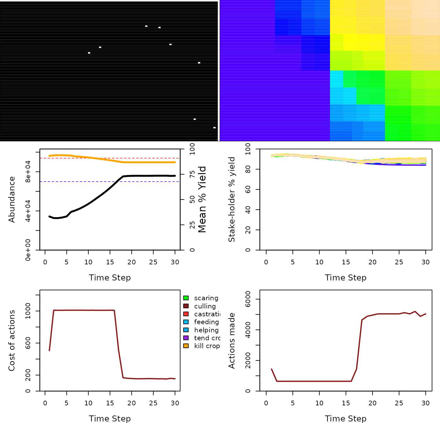

Results of a GMSE simulation using parameters estimated for Taiga Been Geese Central Management Unit. This example includes 80 farmers whose objective is to maximise their agricultural output, and one manager whose objective is to keep geese at a target abundance, over 30 simulated time steps. Goose locations at the end of the simulation are shown in the upper left panel, while the upper right panel shows the same landscape broken down among the 80 farmers (upper 60% of the landscape in multiple colours), along with non-agricultural land (lower 40% of the landscape in blue). Actual goose abundance is shown in the middle left panel (black solid line), along with its estimate by the manager (blue solid line, hidden underneath the black line). The horizontal red and blue dotted lines show goose carrying capacity and the manager’s target for goose abundance, respectively. The orange line shows the total percent of landscape cell (including non-farmed cells) yield, as decreased by geese. The middle right panel shows this yield for each farmer, and for the public land (lower line in blue). The lower left panel shows the cost of culling for farmers, as set by the manager, and the lower right panel shows the total number of culls attempted by farmers over time.

Figure 1 shows the dynamics of goose abundance and agricultural yield, along with how managers react to change in abundance and farmers react to manager policy. In the case of the simulation above, managers quickly set a policy of high cost for culling, which leads to a rise in the goose population and a decrease in crop yield for farmers. After roughly 20 time steps, the goose population rises above the manager target, at which point the manager becomes more permissive of culling and the cost of culling for users therefore declines. In response, users begin to cull geese on their land, and the goose population begins to stabilise around the target of 7000 total geese. We can investigate the conflict between management policy and farmers more directly using the plot_gmse_effort function (Figure 2).

plot_gmse_effort(sim_results = sim_1);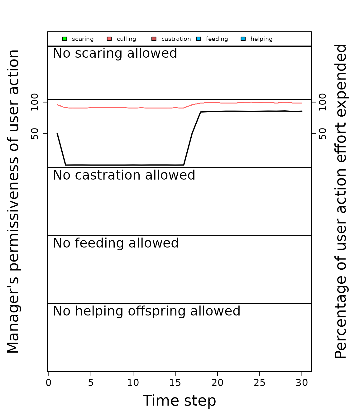

Permissiveness that each manager exhibits for each farmer action (black lines) and the effort that each individual farmer puts into each action over time (coloured lines). Each panel row reports a different action (in decreasing order: scaring, culling, castration, feeding, and helping). The left axis shows the permissiveness that a manager has for the focal action (black line), which is calculated as 100 minus the percent of the manager’s budget that is put into increasing the cost of the focal action. For example, if the manager puts all of their effort (total budget) into increasing the cost of culling, then permissiveness of culling is 0; if the manager puts no effort into increasing culling cost, then permissiveness of culling is 100. The right axis shows effort that farmers put into an action (coloured lines), which defined as the percentage of a farmer’s budget put into a particular action (note, values might not add up to 100 because farmers are not forced to use their entire budget).

Black lines in Figure 2 indicate how permissive a manager is toward a particular action on a scale of 0 to 100, while coloured lines indicate how much effort farmers expend on a given action. When black lines are far below coloured lines, we can (cautiously) interpret this as a conflict between management of the goose population and farmer’s interest in agricultural production. These time periods represent instances in which the manager is not permissive of a particular action (in this case culling), but farmers continue to expend effort to do the action anyway. In the case of the above simulation of potential conflict between farmers and goose conservation, conflict is highest before time step 20, where the manager is not permissive of culling because the population is below the manager’s target. Once the goose population has increased above the manager’s target, conflict decreases because the desired culling is permitted by managers to keep the population at a target abundance. It is worth noting that, despite conflict as we define it decreasing, agricultural damage is still relatively high after the target goose population size is achieved (Figure 1). Hence, on a broader scale, conflict might persist around the appropriate target population size rather than what actions are permitted for farmers; currently, this potential aspect of conflict is not modelled, but future versions of GMSE may attempt to incorporate such additional complexity in conflict scenarios.

We can model the consequences for goose population dynamics, agricultural production, and conservation conflict when scaring is a policy option available to the manager. The code below runs a simulation identical to the one just discussed, but with a scaring option included using the argument scaring = TRUE.

sim_2 <- gmse(manager_budget = 10000, user_budget = 10000, res_death_K = 93870, 
             manage_target = 70000, RESOURCE_ini = 35000, plotting = FALSE, 
             stakeholders = 80, land_ownership = TRUE, public_land = 0.4, 
             scaring = TRUE, lambda = 0.275, remove_pr = 0.122, time_max = 30, 
             res_death_type = 3, res_consume = 0.02, res_birth_K = 200000, 
             observe_type = 3, agent_view = 1, converge_crit = 0.01, 
             ga_mingen = 200);

The results are plotted in Figure 3.

plot_gmse_results(sim_results = sim_2);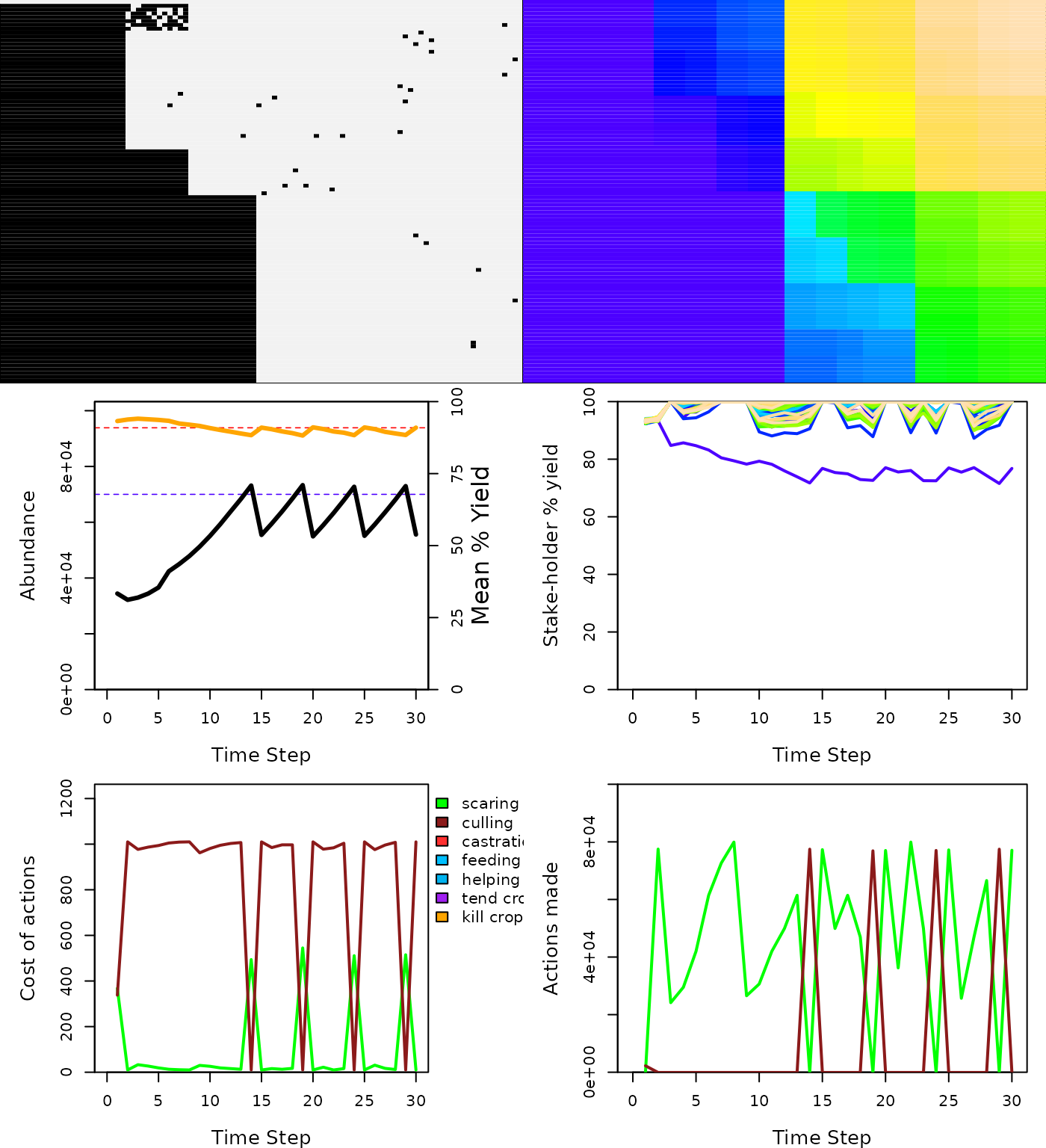

Results of a GMSE simulation using parameters estimated for Taiga Been Geese Central Management Unit in which scaring is permitted. Simulation output is interpreted as in Figure 1.

When scaring is introduced to an otherwise identical simulation (compare Figure 3 to Figure 1), the goose population increases as before, but it achieves the manager’s target population size and stabilises 2-3 time steps earlier. The reason for this earlier stabilisation is due to the change in farmer’s actions as a consequence of the introduced scaring policy. At the start of the simulation, managers adjust policy by quickly increasing the cost of culling and decreasing the cost of scaring. In response, farmers turn to scaring rather than culling to remove geese from their land cells (Figure 3). This is in contrast to the simulation in which scaring was not an option, and farmers simply culled as much as possible despite the high costs (Figure 1). After the population has risen to slightly above the manager’s target, the cost of culling again decreases, with the manager balancing the incentivisation of culling and scaring. The consequence of scaring as an available policy also reveals some potentially unexpected outcomes, such as increased variance in among-farmer agricultural production, which arises as geese are scared from one area of the landscape to another.

We can use the plot_gmse_effort function as before to investigate how the inclusion of scaring as a policy option might affect conservation conflict. Conflict results when scaring is included are plotted in Figure 4.

plot_gmse_effort(sim_results = sim_2);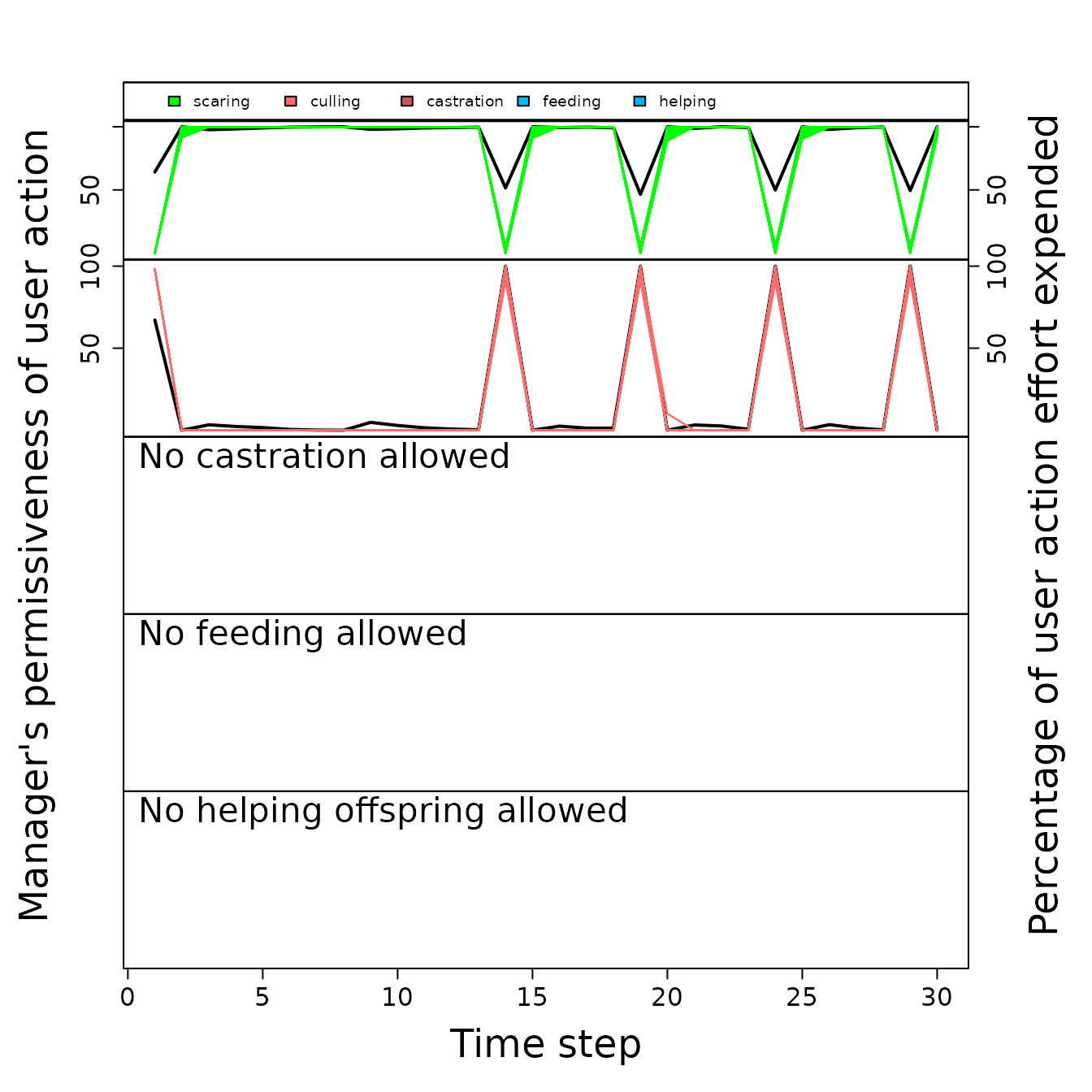

Permissiveness that each manager exhibits for each farmer action (black lines) and the effort that each individual farmer puts into each action over time (coloured lines) given scaring as a possible policy option. Simulation output is intepreted as in Figure 2.

Unlike the case in which culling was the only policy option (compare Figure 4 to Figure 2), the effort that farmers expended on a given action did not rise as highly above the manager’s permissiveness of the action. Hence, under the conditions of this model, the inclusion of scaring as a policy option has reduced conservation conflict in the social-ecological system. We again emphasise that the simulations presented here only serve as an example for how GMSE could be used as a tool for simulating social-ecological systems and understanding the potential for conflict; it is not intended to inform policy in Taiga Bean Geese or any other specific system.

Default and non-default options in default GMSE sub-models

Within the default sub-models of GMSE, there are several non-default options that can be set using arguments to gmse and gmse_apply. Brief explanations of these non-default options appear in the GMSE documentation (also listed on the GMSE website). Here we further explain some of the less obvious or less intuitive options available in GMSE, for which additional explanation beyond the GMSE documentation may be warranted for application to case studies such as the Taiga Bean Geese case study example demonstrated above. Future versions of GMSE are expected to expand upon these options.

res_move_type: Resources in default GMSE sub-models can move on the landscape in one of three ways. These different movement types are listed below, and are taken as arguments to gmse (e.g., gmse(res_move_type = 2)).

0. No movement. Given this option, resources do not move at all in the resource sub-model, and instead remain on the location at which they are initialised.
1. Uniform movement in any direction up to res_movement cells away from a resource’s original location (default). In uniform movement, the resource moves to a new cell within some distance res_movement of its original location in each time step. Distance therefore includes diagonal movement, such that a resource capable of moving res_movement = 1 cell away can go to any of the eight adjacent cells around its current location; it can also remain on its current cell. Similarly, a resource capable of moving res_movement = 2 cells away can go to any of the 24 cells surrounding its current location, or remain on its current cell. The distance (in cells) moved in the x-direction (i.e., left to right) and y-direction (i.e., up and down), is sampled from a uniform distribution, meaning that all reachable cells (including the resource’s current cell) have equal probability of being selected as the resource’s new cell location.
2. Poisson selected movement distance and direction. In this movement type, the distance (in cells) moved in the x-direction and the y-direction are sampled from a Poisson distribution using res_movement as the rate parameter (i.e., the mean movement distance in each direction). Using this movement type is not generally recommended because it is not likely to be biologically realistic (e.g., diagonal movement is rare because selection of both high x-direction and high y-direction values is unlikely).
3. Uniform movement in any direction up to res_movement cells away from a resource’s original location res_movement times. Like option (1), when moving, resources can travel in any direction up to res_movement cells from their current location with equal probability. What is different about this option is that uniform movement in any direction occurs \(C =\) Poisson(res_movement) times. In other words, when a resource moves, it first decides how many different cells it will visit (\(C\)), as determined by sampling from a Poisson distribution with a rate parameter of res_movement (i.e., the mean number of visited cells will be res_movement). Upon leaving a cell, the resource will move in the same way as defined in option (1) above, by choosing a cell within res_movement distance (in cells) of its current cell. It continues moving in this way until \(C\) cells have been visited. This type of movement has been used in some individual-based models of plant-pollinator interactions (e.g., Duthie and Falcy 2013; Wilson, Morris, and Bronstein 2003).

res_birth_type: Resources in GMSE can be added to the model in one of two ways within the default resource sub-model, thereby simulating resource birth. It is important to note that res_birth_type refers only to additions that occur within the resource sub-model; additions from user actions (e.g., the help_offspring option) occur within the user sub-model.

0. No explicit resource addition. This option causes no baseline resource additions, but resource birth is still possible if consume_repr > 0. Under such conditions, landscape yield consumed by the resource will result in floor(yield_consumed / consume_repr) offspring produced. The amount of yield a resource consumes will be affected by both times_feeding (how many times the resource moves and feeds on a new landscape cell during a time step) and res_consume (the proportion of yield on a cell that is consumed upon visit to the cell). Note that consume_repr can still be used when res_birth_type > 0 (below), resulting in multiple sources of resource addition.
1. Fixed number added per resource. For this option, each resource produces lambda new resources in each time step.
2. Poisson sampling. For this option, each resource produces a number of offspring as determined by sampling from a Poisson distribution in which lambda is the rate parameter (i.e., each resource is expected to produce lambda offspring).

res_death_type: Resources in GMSE can be removed from the model in one of four ways within the default resource sub-model, thereby simulating resource death. It is important to note that res_death_type refers only to removal that occurs within the resource sub-model; removal from user actions (e.g., death from shooting) occurs within the user sub-model.

0. No explicit density independent or dependent removal, and no old age. Given this option, the only way in resources can be removed is if users remove them through their actions (i.e., culling). Resources cannot die due to lack of resource consumption, density independent or dependent effects, or old age.
1. Density-independent removal. Given this option, there is no explicit density-dependent removal of resources within the resource sub-model. Resources are simply removed with a fixed probability of removal_pr (its default value is 0) each time the sub-model is run. This option should be used with great care because in the absence of density-dependence, it is possible for the population of resources to increase without limit and thereby greatly slow down simulation times. Usually res_death_type = 1 is most useful when combined with consumption limited survival (consume_surv) and reproduction (consume_repr); see below.
2. Density-dependent removal (default). Given this option, removal of resources within the resource sub-model is caused by density effects. The probability that a resource is removed is a function of the resource carrying capacity set using the res_death_K parameter. If the number of resources (\(N\)) is greater than res_death_K (\(K\)), then the probability that an individual resource is removed is defined by \((N - K) / N\). Removal then occurs independently for each resource based on this probability.
3. Density-independent and density-dependent removal. This option allows a combination of both options (1) and (2), which affect removal independently. In other words, each resource is assigned a probability of removal removal_pr as in (1), and then independently assigned another probability of removal based on res_death_K as in (2). If removal occurs as a consequence of (1), (2), or both, then the resource is removed.

Note that for all res_death_type > 0, removal can occur when the argument consume_surv > 0 (its default value is 0). In this case, survival of a resource in a time step depends on that resource consuming at least consume_surv in yield on the landscape. In such cases, a natural carrying capacity can be generated as more resources result in higher total consumption. The amount of yield that a resource consumes is further affected by both times_feeding (how many times the resource moves and feeds on a new landscape cell during a time step) and res_consume (the proportion of yield on a cell that is is consumed upon visit to the cell). To ensure that resource death is only limited by consumption and user actions, set res_death_type = 1 and removal_pr = 0. Under this scenario, resources will only die if the do not consume enough, are culled by users, or are above the max_age.

observe_type: Observation of resources in default GMSE sub-models can occur in one of four ways. Each observation type mimics some process of resource observation, with potential error affected by observation intensity.

0. Density-based observation. In this option, managers observe resources on a subset of the landscape; subset size is determined by the manager’s view as set using the agent_view parameter. In practice, this is done by having the manager count all of the resources within a distance (in any direction) of agent_view cells of their location. Managers then extrapolate the density of resources within this subset to estimate the total number of resources on the landscape. For example, if the manager has an agent_view of 1, then they are capable of seeing all of the resources on nine landscape cells (the cell on which they are located, and each adjacent cell). If they count that there are 90 resource on these nine cells, then they calculate a resource density of 10 per cell. They then multiply the density of 10 by the total number of landscape cells to estimate the number of resources on the landscape. The error of this estimate naturally decreases with increasing agent_view, such that when the manager is capable of viewing the entire landscape, observation error is zero. If desired, the times_observe (default equals 1) option can also be used to allow managers to sample more than one landscape subset in their estimate (e.g., if times_observe = 2, then density is estimated from two different locations, with the mean of individual estimates used for a combined estimate of population density). Note that if times_observe = 1, then manager estimates might be consistently biased if they are observing from a location with disproportionately many or few resources.
1. Mark-recapture observation. This option simulates the process of a mark-recapture analysis. In this process, managers randomly sample fixed_mark resources in the population; sampling occurs without replacement and without any spatial bias, and if fixed_mark is greater than the total number of resources on the landscape, then managers sample all resources. The manager then randomly samples fixed_recapt resources, again without replacement or spatial bias. The sampled resources from fixed_mark and fixed_recapt are interpreted as marked and recaptured resources, respectively, and a Chapman estimate (Pollock et al. 1990) is then used in the manager model to calculate estimated population size form these observation data. Error in this estimate can be naturally minimised if both fixed_mark and fixed_recapt are very high.
2. Sample linear transect. This option simulates sampling from a linear transect of the landscape. The manager samples an entire set of cell rows on the landscape and counts the total resources on all cells; the manager then continues onto the next set of landscape rows until the entire landscape has been sampled. The number of rows observed in each sample is defined by agent_view. For example, if the landscape is of the dimensions \(100 \times 100\) cells, and agent_view = 2, then the manager will first observe all resources in the upper 200 cells (first \(2 \times 100\) cells in the upper two landscape cell rows), then move onto the next 200 cells, repeating the process 50 times until all rows have been sampled. This process of sampling will only generate observation error if res_move_obs = TRUE, which it is by default. In this case, resources can move on the landscape (according to the rules of res_move_type and distance of res_movement) in between transect observation, potentially causing some resources to escape observation and others to be observed more than once.
3. Sample block transect. This option is identical to the sample linear transect option above, except that instead of sampling an entire row of a landscape, the manager samples one square block of the landscape at a time. The cell length of each block side equals agent_view, meaning that the manager can observe all of the resources on agent_view * agent_view cells at a time. The manager proceeds to observe the entire landscape, block by block, until all cells on the landscape have been covered. For example, if agent_view = 25, and the landscape is of the dimensions \(100 \times 100\), then the manager will sample four total blocks of the landscape, one at a time, and use the total number of resources observed as the estimate of resource density on the landscape. As with linear transect sampling, if res_move_obs = TRUE (which it is by default), then resources can move on the landscape between block samples, potentially causing observation error if some resources are missed due to movement, or counted multiple times.

obs_move_type: Observation of agents (manager and users) in default GMSE sub-models can occur in the same four ways as allowed in res_move_type (default obs_move_type = 1), with movement distance defined by the parameter agent_move (default 50). Currently, the only effect of this movement is to allow for spatially autocorrelated sampling of resources by the manager in the observation model. If the manager is using density-based sampling (observe_type = 0) and sampling more than one subset of the landscape (times_observe > 1), then the manager’s movement between subsets is governed by res_move_type (movement rules) and agent_move (movement distance). Hence, to have the manager observe the population many times in one area of the landscape, the times_observe option should be increased above one and agent_move should be decreased to a low value.

times_feeding: By default, resources feed once at the start of each time step (times_feeding = 1), then move at the end the time step. Consequently, where they move to at the end of the time step will be where they feed at the start of the next time step, which gives users the opportunity to potentially cull or scare them prior to feeding. When times_feeding > 1, at the start of each time step, resource feeding on their cell, then immediately move to a new cell on which to feed. This feeding and moving continues until the resource has fed times_feeding times, at which point on the cell at which they last fed, potentially reproduce, then move again at the end of the time step. Feeding and moving actions happen in a random order for resources so that one resource does not do all of its feeding before another resource has any chance to feed. For example, if there are 10 resources and times_feeding = 4, then the 40 total feeding and moving actions happen in a random order.

Conclusions and future development

The GMSE function gmse and its graphical user interface counterpart gmse_gui offer wide a suite of options for parameterising simulations to fit empirical case studies of conservation interest using default GMSE natural resource, observation, manager, and user sub-models. Future development of these sub-models might usefully incorporate additional details relevant to specific case studies, such population structure, multiple natural resource and user types, or different manager policy and user action possibilities. Requests for new features and contributions to GMSE can be made through GitHub. Additionally, where entirely different types of sub-models are required, the gmse_apply function can be used to more flexibly simulate social-ecological systems. In Advanced case study options, we show an example of this using the same Taiga Bean Geese case study that we did here.

References

AEWA. 2016. “International single species action plan for the conservation of the Taiga Bean Goose (Anser fabalis fabalis).” http://www.unep-aewa.org/sites/default/files/document/aewa_egmp_inf_2_issap_tbg.pdf.

Cusack, Jeremy J, A Bradley Duthie, Sarobidy Rakotonarivo, Rocío A Pozo, Tom H E Mason, Johan Månsson, Lovisa Nilsson, et al. 2018. “Time series analysis reveals synchrony and asynchrony between conflict management effort and increasing large grazing bird populations in northern Europe.” Conservation Letters, e12450. https://doi.org/10.1111/conl.12450.

Duthie, A Bradley, and Matthew R Falcy. 2013. “The influence of habitat autocorrelation on plants and their seed-eating pollinators.” Ecological Modelling 251: 260–70. https://doi.org/10.1016/j.ecolmodel.2012.12.019.

Fox, Anthony D, Bart S Ebbinge, Carl Mitchell, Thomas Heinicke, Tomas Aarvak, Kendrew Colhoun, Preben Clausen, et al. 2010. “Current estimates of goose population sizes in western Europe, a gap analysis and an assessment of trends.” Ornis Svecica 20 (3-4): 115–27. https://doi.org/10.1111/j.1365-2486.2005.00941.x.

Fox, Anthony D, and Jesper Madsen. 2017. “Threatened species to super-abundance: The unexpected international implications of successful goose conservation.” Ambio 46 (s2): 179–87. https://doi.org/10.1007/s13280-016-0878-2.

Johnson, Fred A, Mikko Alhainen, Anthony D Fox, Jesper Madsen, and Matthieu Guillemain. 2018. “Making do with less: Must sparse data preclude informed harvest strategies for European waterbirds.” Ecological Applications 28 (2): 427–41. https://doi.org/10.1002/eap.1659.

Mason, Tom H. E, Aidan Keane, Stephen M Redpath, and Nils Bunnefeld. 2017. “The changing environment of conservation conflict: geese and farming in Scotland.” Journal of Applied Ecology, 1–12. https://doi.org/10.1111/1365-2664.12969.

Pollock, Kenneth H, James D Nichols, Cavell Brownie, and James E Hines. 1990. “Statistical inference for capture-recapture experiments.” Wildlife Monographs 27 (4): 938–42.

Redpath, Steve M, Juliette Young, Anna Evely, William M Adams, William J Sutherland, Andrew Whitehouse, Arjun Amar, et al. 2013. “Understanding and managing conservation conflicts.” Trends in Ecology & Evolution 28 (2): 100–109. https://doi.org/10.1016/j.tree.2012.08.021.

Tulloch, Ayesha I T, Sam Nicol, and Nils Bunnefeld. 2017. “Quantifying the expected value of uncertain management choices for over-abundant Greylag Geese.” Biological Conservation 214: 147–55. https://doi.org/10.1016/j.biocon.2017.08.013.

Wilson, William G, William F Morris, and Judith L Bronstein. 2003. “Coexistence of mutualists and exploiters on spatial landscapes.” Ecological Monographs 73 (3): 397–413.