The Genetic Algorithm of GMSE
GMSE: an R package for generalised management strategy evaluation (Supporting Information 1)
A. Bradley Duthie¹³, Jeremy J. Cusack¹, Isabel L.
Jones¹, Jeroen Minderman¹,
Erlend B. Nilsen², Rocío A. Pozo¹, O. Sarobidy Rakotonarivo¹,
Bram Van Moorter², and Nils Bunnefeld¹
Erlend B. Nilsen², Rocío A. Pozo¹, O. Sarobidy Rakotonarivo¹,
Bram Van Moorter², and Nils Bunnefeld¹
[2] Norwegian Institute for Nature Research, Trondheim, Norway [3] alexander.duthie@stir.ac.uk
Source:vignettes/SI1.Rmd
SI1.RmdExtended introduction to the genetic algorithm applied in GMSE
Game theory is the formal study of strategic interactions, and can therefore be applied to modelling stakeholder actions and addressing issues of cooperation and conflict in conservation (Lee 2012; Kark et al. 2015; Adami, Schossau, and Hintze 2016; Tilman, Watson, and Levin 2016; Redpath et al. 2018). In game-theoretic models, agents adopt strategies to make decisions that maximise some type of payoff (e.g., utility, biological fitness). Agents are constrained in their decision-making, and realised pay-offs depend on decisions made by other agents. In simple models, it is often useful to assume that agents are perfectly rational decision-makers, then find optimal solutions for pay-off maximisation mathematically. But models that permit even moderately complex decision-making strategies or pay-off structures often include more possible strategies than are mathematically tractable (Hamblin 2013). In these models, genetic algorithms, which mimic the process of natural selection (mutation, recombination, selection, reproduction), can find adaptive (i.e., practical, but not necessarily optimal) solutions for game strategies (e.g., Balmann and Happe 2000; Tu, Wolff, and Lamersdorf 2000; Hamblin 2013).
A genetic algorithm is called in the predefined GMSE manager and user
models to simulate human decision making. As of GMSE version 0.6, this
includes one independent call to the genetic algorithm for each
decision-making agent in every GMSE time step. Therefore, one run of the
genetic algorithm occurs to simulate the manager’s policy-setting
decisions in each time step (unless otherwise defined through
non-default manage_freq values greater than 1; e.g., see Management frequency and extinction risk), and one
run occurs to simulate each individual user’s action decisions in each
time step (unless otherwise defined through non-default
group_think = TRUE, in which case one user makes decisions
that all other users copy). Each run of the genetic algorithm mimics the
evolution by natural selection of a population of potential manager or
user strategies over multiple iterations, with the highest fitness
strategy in the terminal iteration being selected as the one that the
manager or user decides to implement. For clarity, as in the main text,
we use ‘time step’ to refer to a full GMSE cycle (in which multiple
genetic algorithms may be run) and ‘iteration’ to refer to a single,
non-overlapping, generation of potential strategies that evolve within a
genetic algorithm (see Figure 1 of the main text).
Below, we explain the genetic algorithm in detail, as it occurs in GMSE
v0.6+ (future versions of GMSE might expand upon this framework, and we
highlight some of these potential avenues for expansion). We first
explain the key data structures
used, then provide an overview of how a population of strategies is
initialised, and the subsequent processes of
crossover, mutation, cost constraint, fitness
evaluation, tournament selection, and replacement. We then explain the fitness
functions of managers and users in more detail.
Key data structures used
The focal data structure used for tracking manager and user decisions
is a three dimensional array, which we will call ACTION
(also returned as user_array by gmse_apply;
see Default GMSE data structure). Rows of
ACTION correspond to the entities affected by actions
(resources, landscape properties, or potentially other agents), and
columns correspond either to properties of the affected entities, or to
the actions potentially allocated to them. Each layer of
ACTION corresponds to a unique agent, the first of which is
the manager; additional layers correspond to users. Below shows an
ACTION array for a GMSE model with one manager and two
users.
## , , Manager_Actions
##
##           Act Type_1 Type_2 Type_3      Util. U_land U_loc. Scare Cull Castrate
## Resource   -2      1      0      0 1000.00000      0      0     0    0        0
## Landscape  -1      1      0      0    0.00000      0      0     0    0        0
## Res_cost    1      1      0      0   24.94331      0      0    10   60       10
## U1_cost     2      1      0      0    0.00000      0      0     0    0        0
## U2_cost     3      1      0      0    0.00000      0      0     0    0        0
##           Feed Help_off None
## Resource     0        0    0
## Landscape    0        0    0
## Res_cost    10       10   60
## U1_cost      0        0    0
## U2_cost      0        0    0
##
## , , User_1_Actions
##
##           Act Type_1 Type_2 Type_3 Util. U_land U_loc. Scare Cull Castrate Feed
## Resource   -2      1      0      0    -1      0      0     0   16        0    0
## Landscape  -1      1      0      0     0      0      0     0    0        0    0
## Res_cost    1      1      0      0     0      0      0     0    0        0    0
## U1_cost     2      1      0      0     0      0      0     0    0        0    0
## U2_cost     3      1      0      0     0      0      0     0    0        0    0
##           Help_off None
## Resource         0    0
## Landscape        0    1
## Res_cost         0    0
## U1_cost          0    0
## U2_cost          0    0
##
## , , User_2_Actions
##
##           Act Type_1 Type_2 Type_3 Util. U_land U_loc. Scare Cull Castrate Feed
## Resource   -2      1      0      0    -1      0      0     0   16        0    0
## Landscape  -1      1      0      0     0      0      0     0    0        0    0
## Res_cost    1      1      0      0     0      0      0     0    0        0    0
## U1_cost     2      1      0      0     0      0      0     0    0        0    0
## U2_cost     3      1      0      0     0      0      0     0    0        0    0
##           Help_off None
## Resource         0    0
## Landscape        0    2
## Res_cost         0    0
## U1_cost          0    0
## U2_cost          0    0
The above array holds all of the information on manager and user
actions. The first seven columns contain information about which
entities are affected, and how they are affected. The first column
Act identifies the type of action being performed; a value
of -2 defines a direct action to a resource (e.g., culling of the
resource), and a value of -1 defines direct action to a landscape (e.g.,
increasing yield). Positive values are currently only meaningful for
Manager_Actions, where a value of 1 defines an action
setting a uniform cost of users’ direct actions on resources (i.e.,
costs where Act = -2 for User_1_Actions and
User_2_Actions). All other values for Act are
meaningless in GMSE 0.6, but might be expanded upon in future versions
to allow for modification of specific user costs enacted by managers
(i.e., managers having different policies for different users) or other
users (e.g., users increasing the costs of other users’ actions due to
conflict or cooperation). We will therefore focus only on rows 1-3 of
ACTION.
Columns 2-4 refer to resource or landscape types, but only
Type_1 = 1, Type_2 = 0, and
Type_3 = 0 are allowed in predefined GMSE v0.6+ manager and
user sub-models (i.e., only one type of resource is permitted). Future
versions might allow for different resource types (e.g.,
Type_1 might be used to designate species, and
Type_2 and Type_3 could designate stage or
sex). Column 5 Util. of ACTION defines the
utility associated with the resource (where Act = -2) or
landscape (where Act = -1). For managers, the target
resource abundance set with the GMSE argument manage_target
is found in row 1 (1000 in ACTION above); for users, the
value in row 1 identifies whether resources are preferred to increase
(if positive) or decrease (if negative). Values of column 5 in row 2
similarly identify whether landscape cell output is preferred by users
to increase or decrease (managers do not currently have preferences for
landscape output). Of special note is row 3 for
Manager_Actions, which defines the current
manager’s utility for resources; that is, the adjustment to resource
abundance that the manager will attempt to make based on the
manage_target and the most recent estimate of resource
abundance produced by the observation model (in the case of the above,
resource abundance is estimated at ca 975.06, so the manager will set
policy in attempt to change the population size by ca 24.94 resources).
Column 6 U_land defines whether or not the utility attached
to the resource or landscape output depends on it being on a landscape
cell that is owned by the acting user. Related, column 7
U_loc. defines whether or not actions can be performed only
on a landscape cell that is owned by the acting user. Hence values of
columns 6 and 7 are binary, and affected by the
land_ownership argument in gmse and
gmse_apply. Finally, columns 8-13 correspond to specific
actions, either direct (where Act < 0) or indirect by
setting policy (for row 3 of Manager_Actions where
Act = 1). The last column 13 None corresponds
with no actions. See GMSE
documentation for details about the effects of each action.
Constraints on the values that elements in the ACTION
array can take are defined by a COST array (also returned
as manager_array by gmse_apply; see Default GMSE data structures) of dimensions
identical to ACTION. Elements of COST define
how many units from the manager_budget or
user_budget are needed to perform a single action; a
minimum_cost for actions is defined as an argument in GMSE
(10 by default). All values in COST columns 1-7 are set to
100001, one higher than the highest possible manager_budget
or user_budget, so neither managers nor users can affect
resource types or utilities. Columns 8-13 are also set to 100001, except
where actions are allowed. Maximum values of 100000 are independent of
any other parameter value specified in GMSE (e.g., landscape
dimensions). Below shows the COST array that corresponds to
the above ACTION array.
## , , Manager_Costs
##
##              Act Type_1 Type_2 Type_3  Util. U_land U_loc.  Scare   Cull
## Resource  100001 100001 100001 100001 100001 100001 100001 100001 100001
## Landscape 100001 100001 100001 100001 100001 100001 100001 100001 100001
## Res_cost  100001 100001 100001 100001 100001 100001 100001 100001     10
## U1_cost   100001 100001 100001 100001 100001 100001 100001 100001 100001
## U2_cost   100001 100001 100001 100001 100001 100001 100001 100001 100001
##           Castrate   Feed Help_off   None
## Resource    100001 100001   100001     10
## Landscape   100001 100001   100001     10
## Res_cost    100001 100001   100001     10
## U1_cost     100001 100001   100001 100001
## U2_cost     100001 100001   100001 100001
##
## , , User_1_Costs
##
##              Act Type_1 Type_2 Type_3  Util. U_land U_loc.  Scare   Cull
## Resource  100001 100001 100001 100001 100001 100001 100001 100001     60
## Landscape 100001 100001 100001 100001 100001 100001 100001 100001 100001
## Res_cost  100001 100001 100001 100001 100001 100001 100001 100001 100001
## U1_cost   100001 100001 100001 100001 100001 100001 100001 100001 100001
## U2_cost   100001 100001 100001 100001 100001 100001 100001 100001 100001
##           Castrate   Feed Help_off   None
## Resource    100001 100001   100001     10
## Landscape   100001 100001   100001     10
## Res_cost    100001 100001   100001 100001
## U1_cost     100001 100001   100001 100001
## U2_cost     100001 100001   100001 100001
##
## , , User_2_Costs
##
##              Act Type_1 Type_2 Type_3  Util. U_land U_loc.  Scare   Cull
## Resource  100001 100001 100001 100001 100001 100001 100001 100001     60
## Landscape 100001 100001 100001 100001 100001 100001 100001 100001 100001
## Res_cost  100001 100001 100001 100001 100001 100001 100001 100001 100001
## U1_cost   100001 100001 100001 100001 100001 100001 100001 100001 100001
## U2_cost   100001 100001 100001 100001 100001 100001 100001 100001 100001
##           Castrate   Feed Help_off   None
## Resource    100001 100001   100001     10
## Landscape   100001 100001   100001     10
## Res_cost    100001 100001   100001 100001
## U1_cost     100001 100001   100001 100001
## U2_cost     100001 100001   100001 100001
Note that in default GMSE parameters, culling = TRUE,
but all other actions are set to FALSE. Hence, the
Cull column 9 is the only column besides column 13
None in which cost is less than 100001. Manager’s actions
in ACTION directly affect the cost of users performing one
of the five possible actions on resources (columns 8-12). This can be
verified in ACTION where the manager has set the cost of
culling to 60 (row 3), and the corresponding COST of
resource culling is 60 for both users (row 1). The cost of the manager
affecting the cost of user actions is always set to the
minimum_cost; here the default 10 is used. This
minimum_cost also defines cost values for
None, in which the user or manager does nothing, as might
occur if the manager wants to permit culling and therefore does not want
to invest any of their manager_budget to increasing the
cost of culling. Both ACTION and COST are
updated in each time step unless manage_freq > 1, in
which case COST and Manager_Actions in
ACTION are updated at the frequency defined.
General overview of key aspects of the genetic algorithm
The genetic algorithm updates a single layer of the
ACTION array, which defines the decisions of a single agent
(either the manager or a user). The corresponding layer of the
COST array remains unchanged, and serves only to ensure
that ACTION values do not exceed
manager_budget or user_budget for managers and
users, respectively. The genetic algorithm proceeds by first
initialising a large (but temporary) population of new
ACTION layers. In each iteration, these layers crossover
and mutate, generating variation in potential agent decisions; costs
constrain this variation from exceeding a maximum budget, then the
fitness of each layer is evaluated based on how the layer is predicted
to affect resources or landscape output to which the agent has assigned
some utility. A tournament is used to select high fitness layers, and
these selected layers become the new iteration of layers; iterations
continue until a minimum number of iterations (ga_mingen)
have passed and a convergence criteria is satisfied such that the
increase in mean fitness from the previous iteration is below the
threshold converge_crit (Figure 1 below).
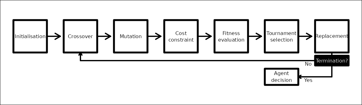
Conceptual overview of the GMSE genetic algorithm
Initialisation
At the start of each genetic algorithm, a population of size
ga_popsize is initialised (hereafter the
POPULATION array). This population is held in a 3D array of
ga_popsize layers. Each layer includes an identical number
of rows and columns as in ACTION, and one layer defines a
single ‘individual’ in the population. The first seven columns of
ACTION are replicated exactly for all individuals, and
remain unchanged throughout the genetic algorithm thereby preserving the
information about which entities are affected by actions in a given row.
The remaining columns are either also replicated exactly as in
ACTION (i.e., initialised to be the same decisions as in a
previous time step), or randomly seeded with values given the
constraints of manager_budget or user_budget
(i.e., initialised to random decision making). The number of exact
replicates initialised is set using ga_seedrep (if
ga_seedrep \(\geq\)
ga_popsize, then all individuals are seeded as replicates).
After the POPULATION of ga_popsize individuals
is initialised, a loop simulating the adaptive evolution of
POPULATION in non-overlapping iterations begins (see Figure
1 above).
Crossover
A single iteration of the genetic algorithm begins with a uniform
crossover (Hamblin 2013), by which actions of
individuals in POPULATION are randomly swapped with some
probability. To implement crossover, each individual selects a partner,
then exchanges corresponding array elements affecting agent actions
(columns 8-13) with their partner at a fixed probability of
ga_crossover.
Mutation
Following crossover, POPULATION array elements affecting
agent actions (columns 8-13) mutate at a fixed probability of
ga_mutation. For each array element, a random uniform
number \(u \in [0, 1]\) is sampled. If
\(u\) is greater than
1 - (0.5 * ga_mutation), then the value of the array
element is increased by 1. If \(u\) is
less than 0.5 * ga_mutation, then the value of the array
element is decreased by 1; when this decrease results in a negative
value, the mutated value is multiplied by -1 to be positive.
Cost constraint
Variation in manager or user actions generated by crossover and
mutation might result in strategies that exceed
manager_budget or user_budget, respectively.
Left unchecked, this over-budgeting could lead to unnacceptably high
fitness strategies, so strategies that are over budget following
crossover and mutation need to be brought back within budgetary
constraints. To do this, the genetic algorithm first checks to see if an
individual in POPULATION is over budget. If so, then an
action is randomly selected and removed, and budget use is reassessed;
this random removal of an action and subsequent budget reassessment
continues until the individual does not exceed their budget.
Fitness evaluation
Once all individuals in POPULATION are within budget,
the fitness of each individual is assessed. Fitness assessment works
differently for managers versus users because managers need to consider
the consequences of their decisions on user actions, and how those
actions will affect resource abundance. In contrast, user actions need
to consider the consequences of their decisions on resource abundance or
landscape output. Individual fitness is defined by a real number that
increases with the degree to which an individual’s actions are predicted
to increase entities of positive utility and decrease entities of
negative utility (recall that managers and users assign resources or
landscape output a utility value). Details for how fitness is calculated
are provided below.
Tournament selection
After each individual in POPULATION is assigned a
fitness, a tournament is used to select individuals. Tournament
selection is an especially flexible, non-parametric method that samples
a subset of individuals from the total population and chooses the
fittest of the subset for replacement (Hamblin 2013).
In GMSE, tournament selection proceeds by randomly sampling
ga_sampleK individuals from the total
POPULATION with replacement. The fitnesses of the subset of
ga_sampleK individuals are compared, and the
ga_chooseK individuals of highest fitness are retained (if
ga_sampleK \(\geq\)
ga_chooseK, then all ga_sampleK are chosen,
but this will prevent adaptive evolution and is therefore not
recommended). Tournaments selecting ga_chooseK individuals
from random subsets of size ga_sampleK continue until a
total of ga_popsize individuals are retained.
Replacement and termination
Once a new set of ga_popsize individuals is retained
through tournament selection, these individuals replace the previous
POPULATION array. The genetic algorithm terminates if and
only if a minimum number of iterations has passed
(ga_mingen) and a convergence criteria
(converge_crit) is satisfied. The convergence criteria
checks the difference between the mean fitness of individuals in the new
iteration versus the previous iteration; if this difference is greater
than converge_crit, then termination does not occur (this
prevents termination from occuring while fitness is still increasing,
though it is usually fine to use the default GMSE
converge_crit = 0.1 and ga_mingen = 40, which
nearly always terminates the genetic algorithm after 40 iterations
having identified adaptive manager or user strategies). Due to the way
in which fitness is calculated (see below), in practice,
converge_crit currently applies only to users. If
termination conditions are not satisfied, then the
POPULATION of individuals begins a new iteration of
crossover, mutation, cost constraint, fitness evaluation, and tournament
selection (Figure 1).
Detailed explanation of manager and user fitness functions
Here we explain how the fitnesses of candidate manager and user
strategies in a POPULATION array (see above) are
calculated. We emphasise that the fitness functions used in GMSE v0.6+
are intended to be heuristic tools for identifying reasonable manager
and user behaviours. In practice, our fitness functions identify
behaviours that are well-aligned with manager and user interests for
harvesting or crop yield, but they are not intended to identify
optimal decisions. This practical, metaheuristic approach is
consistent with the objectives of management strategy evaluation (Bunnefeld et al. 2011), and is
well-suited for the use of genetic algorithms (Hamblin 2013).
(Luke2009?) describes
the metaheuristic approach more generally (original emphasis
retained):
Metaheuristics are applied to I know it when I see it problems. They’re algorithms used to find answers to problems when you have very little to help you: you don’t know beforehand what the optimal solution looks like, you don’t know how to go about finding it in a principled way, you have very little heuristic information to go on, and brute-force search is out of the question because the space is too large. But if you’re given a candidate solution to your problem, you can test it and assess how good it is. That is, you know a good one when you see it.
Given the complexity of adaptive management and socio-ecological interactions, the above conditions for applying the metaheuristic approach are clearly satisfied for manager and user decisions. With this in mind, we now explain the details of manager and user fitness functions; that is, how GMSE assesses whether or not a strategy is a good one.
Fitness function for managers
Individual fitness as calculated for managers (\(F_{i}^{m}\)) is affected by a manager’s
utility for resources and the projected change in resource abundance
caused by the individual’s policy (i.e., the contents of their
POPULATION layer, specifically row 3; here again we use
‘individual’ to refer to one of ga_popsize discrete
strategies in POPULATION, which may be selected and
reproduce within the genetic algorithm). Manager utility for a resource
(\(U^{m}_{res}\)) is defined as the
difference between manage_target and the estimation of
population abundance as produced by the GMSE observation model (see “Key data structures used” above,
and Default GMSE data structures for more
information). Manager utility can therefore change in each GMSE time
step as estimated resource abundance changes; when the estimated
resource abundance is greater than manage_target, \(U^{m}_{res}\) is negative, and when the
estimated resource abundance is less than manage_target,
\(U^{m}_{res}\) is positive. To get the
fitness of individuals, first the change in resource abundance predicted
by the individual’s policy (\(\Delta
A_{i}\)) is calculated, then the squared difference between \(\Delta A_{i}\) and \(U^{m}_{res}\) is calculated to obtain a
utility deviation (\(D_{i}\)) for the
individual \(i\),
\[ D_{i} = (\Delta A_{i} - U^{m}_{res})^2. \]
The value of \(D_{i}\) increases as
\(\Delta A_{i}\) gets further from
\(U^{m}_{res}\); i.e, \(D_{i}\) is high when \(i\) sets a policy that is not predicted to
get closer to the manage_target abundance. Fitness is
defined by first finding the maximum \(D_{i}\) value among all
ga_popsize individuals (\(D_{max}\)), then subtracting \(D_{i}\) from this value for each
individual,
\[ F^{m}_{i} = D_{max} - D_{i}. \]
We have explained how \(U^{m}_{res}\) is calculated in the above section on key data structures. We now explain in more detail how individuals in the genetic algorithm calculate how their actions will affect \(\Delta A_{i}\).
To predict change in resource abundance as a consequence of policy,
an individual first needs to know the total number of actions of all
types \(j\) (e.g., scaring, culling,
etc.) performed by users in the previous time step (\(X_{\bullet, j}\); note that this value
includes the increment manage_caution, with a default of
manage_caution = 1, to ensure that managers do not naïvely
assume that users will not perform an action just because they did not
perform it in the previous time step), and the cost of performing each
action (\(C_{\bullet, j}\)). This
information is collected from ACTION and COST
arrays. The individual \(i\) then needs
to predict how their policy (i.e., the costs that they set for users to
perform an action) will affect the new total number of each action \(j\) performed (\(X_{i,j}\)). To do this, the individual
assumes that total user actions performed under their policy will change
in proportion to that of the old policy, while also recognising that
users have a maximum above which higher costs set by the manager will
have no effect. Interested readers might wish to examine the short new_act
function, which is summarised mathematically below; this function is
called by the policy_to_counts
function in the genetic
algorithm source file.
The manager first calculates how much total budget, as summed over all users, was devoted to an action by multiplying the old per action cost \(C_{\bullet, j}\) by the total number of actions performed, \(X_{\bullet, j}\). The manager then divides this by the new cost \(C_{i, j}\) per action to calculate the new predicted number of actions,
\[X_{i, j} = \frac{X_{\bullet, j} \times C_{\bullet, j}}{C_{i, j}}.\]
Note again that if \(C_{i, j} = C_{\bullet, j}\), then the total number of new predicted actions \(j\) will remain unchanged. If \(C_{i, j} > C_{\bullet, j}\), then the total number of new actions will decrease, and if \(C_{i, j} < C_{\bullet, j}\), then the total number of new actions will increase.
The predicted consequences of \(X_{i,j}\) for resource abundance differ for
each possible action. For each action, no consequence is predicted if
the policy is not allowed by a simulation of GMSE (e.g.,
culling = FALSE). For allowed actions, the parameter
manager_sense (\(\sigma\))
modulates predicted consequences for abundance by some factor; this is
useful because not all actions attempted by users will be realised, and
a value of \(\sigma = 1\) tends to
slightly overestimate how much the actions attempted by users will
actually translate to a change in resource abundance. In practice, the
default \(\sigma = 0.9\) usually
performs well. Managers also have access to an estimate of the number of
offspring that resources produce (\(E[offspring]\)). For default settings in
GMSE v0.6+, \(E[offspring] = \lambda\),
where \(\lambda\) is the GMSE argument
lambda that defines the baseline population growth rate of
resources. Given a non-default GMSE argument for
consume_repr (where consume_repr is how much
consumption of landscape yield is needed to increment offspring
production by 1), \(E[offspring]\) is
further incremented by
( (times_feeding * res_consume) / consume_repr) to account
for reproduction enabled by feeding on the landscape
(res_consume is the proportion of landscape yield that a
resource consumes during feeding).
Allowed actions are predicted by managers to have the following effects (again, we emphasise that whether or not these effects are realised will depend later on the user model, to which the manager – by design – does not have access):
-
scaringis assumed to be nonlethal and therefore have no effect on resource number (resources are moved to a random cell on the landscape, as sampled from a uniform distribution such that movement to any given cell is equally probable). -
cullingdecreases resource number by \(\sigma (1 + E[offspring])\). -
castrationdecreases resource number by \(\sigma (E[offspring])\). -
feedingincreases resource number by \(\sigma (E[offspring])\). -
help_offspringincreases resource number by \(\sigma\).
Note that \(\sigma\) is included in all of the predicted actions above as a modulator for how strongly the manager predicts users will respond to a change in manager policy (e.g., a value of 0 would predict no reaction on the part of users to a change in policy, while a value of 1 would predict that an action would increase in exact proportion to its decrease in cost).
The above effects cannot be altered directly in gmse or
gmse_apply (though parameter values can of course be
changed using manager_sense and arguments affecting \(E[offspring]\)), but future versions of
GMSE might include different predicted effects to increase precision or
allow for multiple resource types or different actions. The summation of
\(X_{i,j}\) for all actions defines the
predicted change in resource abundance caused by the policy of an
individual \(i\), \(\Delta A_{i}\).
Fitness function for users
The previous section described the fitness function applied when individual’s fitness was evaluated for managers; here we explain a separate fitness function that is applied when individuals are instead evaluated for users. Individual fitness as calculated for users (\(F_{i}^{u}\)) is affected by a user’s utility for resources (\(U^{u}_{res}\)) and landscape output (\(U^{u}_{land}\)), and the predicted change in each caused by the user’s actions (\(\Delta A_{i}\) and \(\Delta L_{i}\) for predicted change in resource abundance and summed values of the landscape cells owned by \(i\), respectively). Individual fitness is defined for users below,
\[F_{i}^{u} = \Delta A_{i} U^{u}_{res} + \Delta L_{i} U^{u}_{land}. \]
Note that \(F_{i}^{u}\) increases
when \(\Delta A_{i}\) and \(\Delta L_{i}\) are of the same sign as
\(U^{u}_{res}\) and \(U^{u}_{land}\), respectively. Further, in
GMSE v0.6+, only one term of the equation is nonzero. When
land_ownership = FALSE (default, modelling users that
harvest resources), \(U^{u}_{res} =
-1\) and \(U^{u}_{land} = 0\),
and when land_ownership = TRUE, \(U^{u}_{res} = 0\) and \(U^{u}_{land} = 100\) (modelling farmers
trying to increase crop yield). Hence users only have a single objective
of either decreasing resource abundance or increasing landscape output,
though landscape output might be increased indirectly by decreasing
resource abundance if res_consume > 0.
Unlike the manager fitness function, the
predicted effects of user actions can be defined directly in
gmse and gmse_apply. Hence, it is possible to
specify how effective a user believes, e.g., culling or scaring to be
with respect to their own utility. Arguments to do this include
perceive_scare, perceive_cull,
perceive_cast, perceive_feed,
perceive_help, perceive_tend and
perceive_kill. Each of these arguments define how much a
user believes one action will affect either the user or the landscape.
For example, if perceive_scare = -1, then a user will
perceiving scaring as decreasing the number of resources feeding on
their landscape by 1. A value of perceive_feed = 0.5 would
correspond to a user perceiving feeding to increase the number of
resources by one half. Landscape effects (perceive_tend and
perceive_kill) refer to effects of actions on the
landscape, such that perceive_tend = 0.2 would mean that a
single action of tending crops (i.e., action taken on a single landscape
cell) is perceived to increase crop yield by 0.2, while
perceive_kill = -1 would mean that a single action of
killing crops will remove all yield on the landscape cell.
By default, arguments affecting how users perceive the efficacy of
their own actions are set to NA. Default values are then
calculated from other arguments specified in gmse or
gmse_apply. Default user actions are predicted to affect
resources in the following way (in the below \(E[offspring]\) is calculated in the same
way as in the manager’s fitness function):
-
scaringdecreases resource number by \(1\) times one minus the number of landscape cells that the user owns (i.e.,perceive_scare = -1 * (1 - pr_cells_owned)). This accounts for the increasing probability that resource will be scared back to another landscape cell owned by the focal user. If a user owns no cells, then scaring is assumed to have no effect. -
cullingdecreases resource number by \(1 + E[offspring]\) (i.e.,perceive_cull = -1 * (1 + E_off)). -
castrationdecreases resource number by \(E[offspring]\) (i.e.,perceive_cast = -1 * E_off). -
feedingincreases resource number by \(E[offspring]\) (i.e.,perceive_feed = E_off). -
help_offspringincreases resource number by 1 (i.e.,perceive_help = 1).
The number of each action performed is multiplied by its effect, and the sum of all these products is the predicted \(\Delta A_{i}\),
\[\Delta A_{i} = (\lambda) Feeds + Helps - Scares - (1 + \lambda)Culls - (\lambda) Castrations.\]
There are only two possible actions that users can take to directly
affect landscape output, tending crops (tend_crops) and
killing crops (kill_crops). The increase in landscape
output is modulated by the parameter tend_crop_yld (\(\phi\)). User actions are therefore
predicted to have the following effects for one landscape cell:
-
tend_cropswill increase landscape output by \(\phi\) (i.e.,perceive_tend = tend_crop_yld). -
kill_cropswill decrease landscape output by 1 (since the output of a cell is 1 by default, this action removes all output on a landscape cell; i.e.,perceive_kill = -1).
Actions on resources can also have indirect effects on \(\Delta L_{i}\) when resources consume
output on the landscape; we define the value res_consume as
\(r\). The predicted \(\Delta L_{i}\) is then,
\[\Delta L_{i} = (\phi)Tends - Kills - r\Delta A_{i}.\]
That is, the change in landscape output equals the increase in output from tending crops, minus the number of crops destroyed, minus the change in resource abundance times the effect that resource abundance has on landscape output (note that if user actions decrease resource abundance, then this last term will be positive, increasing landscape output).
Choosing genetic algorithm parameter values
Options for adjusting genetic algorithm parameter values in
gmse and gmse_apply are shown below.
| GMSE argument | Default | Description |
|---|---|---|
ga_popsize |
100 | The number of individuals in the population temporarily simulated during a single run of the genetic algorithm. |
ga_mingen |
40 | The minimum number of iterations that a genetic algorithm will run before settling on an agent’s strategy. |
ga_seedrep |
20 | The number of individuas in the population to be initiaised with the current agent’s strategy (e.g., from a previous time step in the broader GMSE simulation), as opposed to being initialised with random strategies. |
ga_sampleK |
20 | For the tournament step of the genetic agorithm, how many strategies are selected at random from the larger population (with replacement) to be included a the tournament. |
ga_chooseK |
2 | Four the tournament step of the genetic agorithm, how many strategies are selected as winners of the tournament, to be included in the next iteration. |
ga_mutation |
0.1 | The mutation rate of any action in an agent’s strategy |
ga_crossover |
0.1 | The crossover rate of any action in an agent’s strategy; crossover events occur with a different randomly selected strategy in the population. |
ga_converge_crit |
0.1 | The percent increase in strategy fitness from one iteration to the next below which the convergence criteria is satisfied. Iterations wil continue as long as fitness increase is above this convergence criteria. |
group_think |
FALSE | Whether or not all users (i.e., not including the manager) have identical strategies. If TRUE, then one genetic algorithm will be run and applied to all users. |
Given the heuristic goals of the genetic algorithm to mimic the
goal-oriented behaviour of agents, default parameters are typically
sufficient for agent decision making. Key parameters can be adjusted if
more precision in decision making is desired, but these adjustments will
come at a cost of simulation efficiency. For example, increasing
ga_popsize or ga_mingen, or decreasing
ga_converge_crit, might fine tune strategies more
effectively, but this will cause the genetic algorithm to take longer
every time that it is run, ultimately slowing down GMSE simulations.
Alternativey, setting group_think = TRUE will greatly speed
up GMSE simulations when many users are being simulated, but this comes
at the cost of among-user variation in decision making. Overall, we
recommend first using default values in the genetic algorithm before
exploring how other parameter value options affect simulation dynamics;
for a more general discussion about selecting parameter values in
genetic algorithms, see Hamblin (2013).
Future development of fitness functions
The fitness functions defined above are useful heuristics for
simulating manager and user decision-making in a way that produces
realistic, I know it when I see it, strategies. Future versions
of GMSE might improve upon these heuristics to generate more accurate or
more realistic models of human decision making. Such improvements could
incorporate additional information such as memory of actions from
multiple past time steps, or a continually updated estimate for how
actions are predicted to affect resource abundance or landscape output
in a simulation (e.g., through a dynamic manager_sense).
Alternatively, future improvements could usefully incorporate knowledge
of human decision making collected from empirical observation of human
behaviour during conservation conflicts. While such possibilities could
be useful for future GMSE modelling, repeated simulations demonstrate
the ability of the current GMSE genetic algorithm to find adaptive
strategies for managers attempting to keep resources at target
abundance, and users attempting to maximise their harvests or crop
yields. It is therefore useful as a tool for modelling manager and user
decisions in a generalised management strategy evaluation framework.