Advanced case study options
GMSE: an R package for generalised management strategy evaluation (Supporting Information 4)
A. Bradley Duthie¹³, Jeremy J. Cusack¹, Isabel L.
Jones¹, Jeroen Minderman¹,
Erlend B. Nilsen², Rocío A. Pozo¹, O. Sarobidy Rakotonarivo¹,
Bram Van Moorter², and Nils Bunnefeld¹
Erlend B. Nilsen², Rocío A. Pozo¹, O. Sarobidy Rakotonarivo¹,
Bram Van Moorter², and Nils Bunnefeld¹
[1] Biological and Environmental Sciences, University of Stirling, Stirling, UK [2] Norwegian Institute for Nature Research, Trondheim, Norway [3] alexander.duthie@stir.ac.uk
Source:vignettes/SI4.Rmd
SI4.RmdFine-tuning simulation conditions using gmse_apply
Here we demonstrate how simulations in GMSE can be more fine-tuned to
specific empirical situations through the use of
gmse_apply. To do this, we use the same scenario described
in Example case study in GMSE; we first recreate
the basic scenario run in gmse using
gmse_apply, and then build in additional modelling details
including (1) custom placement of user land, (2) parameterisation of individual user budgets, and (3)
density-dependent movement of resources. We
emphasise that these simulations are provided only to demonstrate the
use of GMSE, and specifically to show the flexibility of the
gmse_apply function, not to accurately recreate the
dynamics of a specific system or make management recommendations.
We reconsider the case of a protected waterfowl population that exploits agricultural land (e.g., Fox and Madsen 2017; Mason et al. 2017; Tulloch, Nicol, and Bunnefeld 2017; Cusack et al. 2018). The manager attempts to keep the watefowl at a target abundance, while users (farmers) attempt to maximise agricultural yield on the land that they own. We again parameterise our model using demographic information from the Taiga Bean Goose (Anser fabalis fabalis), as reported by Johnson et al. (2018) and AEWA (2016). Relevant parameter values are listed in the table below.
| Parameter | Value | Description |
|---|---|---|
remove_pr |
0.122 | Goose density-independent mortality probability |
lambda |
0.275 | Expected offspring production per time step |
res_death_K |
93870 | Goose carrying capacity (on adult mortality) |
RESOURCE_ini |
35000 | Initial goose abundance |
manage_target |
70000 | Manager’s target goose abundance |
res_death_type |
3 | Mortality (density and density-independent sources) |
Additionally, we continue to use the following values for
consistency, except in the case of stakeholders, where we
reduce the number of farmers to stakeholders = 8. This is
done to for two reasons. First, it speeds up simulations for the purpose
of demonstration; second, it makes the presentation of our custom
landscape ownership easier to visualise (see below).
| Parameter | Value | Description |
|---|---|---|
manager_budget |
10000 | Manager’s budget for setting policy options |
user_budget |
10000 | Users’ budgets for actions |
public_land |
0.4 | Proportion of the landscape that is public |
stakeholders |
8 | Number of stakeholders |
land_ownership |
TRUE | Users own landscape cells |
res_consume |
0.02 | Landscape cell output consumed by a resource |
observe_type |
3 | Observation model type (survey) |
agent_view |
1 | Cells managers can see when conducting a survey |
All other values are set to GMSE defaults, except where specifically noted otherwise.
Re-creating gmse simulations using
gmse_apply
We now recreate the simulations in Example case
study in GMSE, which were run using the gmse function,
in gmse_apply. Doing so requires us to first initialise
simulations using one call of gmse_apply, then loop through
multiple time steps that again call gmse_apply; results of
interest are recorded in a data frame (sim_sum_1).
Following the protocol introduced in Use of the
gmse_apply function, we can call the initialising simulation
sim_old, and use the code below to read in the relevant
parameter values.
sim_old  <- gmse_apply(get_res = "Full", remove_pr = 0.122, lambda = 0.275,
                       res_death_K = 93870, RESOURCE_ini = 35000,
                       manage_target = 70000, res_death_type = 3,
                       manager_budget = 10000, user_budget = 100000,
                       public_land = 0.4, stakeholders = 8, res_consume = 0.02,
                       res_birth_K = 200000, land_ownership = TRUE,
                       observe_type = 3, agent_view = 1, converge_crit = 0.01,
                       ga_mingen = 200);
Note that the argument get_res = "Full" causes
sim_old to retain all of the relevant data structures for
simulating a new time step and recording simulation results. This
includes the key simulation output, which is located in
sim_old$basic_output, which is printed below.
## $resource_results
## [1] 34219
##
## $observation_results
## [1] 34219
##
## $manager_results
##          resource_type scaring culling castration feeding help_offspring
## policy_1             1      NA     509         NA      NA             NA
##
## $user_results
##         resource_type scaring culling castration feeding help_offspring
## Manager             1      NA       0         NA      NA             NA
## user_1              1      NA     196         NA      NA             NA
## user_2              1      NA     196         NA      NA             NA
## user_3              1      NA     196         NA      NA             NA
## user_4              1      NA     196         NA      NA             NA
## user_5              1      NA     196         NA      NA             NA
## user_6              1      NA     196         NA      NA             NA
## user_7              1      NA     196         NA      NA             NA
## user_8              1      NA     196         NA      NA             NA
##         tend_crops kill_crops
## Manager         NA         NA
## user_1          NA         NA
## user_2          NA         NA
## user_3          NA         NA
## user_4          NA         NA
## user_5          NA         NA
## user_6          NA         NA
## user_7          NA         NA
## user_8          NA         NA
We can then loop over 30 time steps to recreate the simulations from
Example case study in GMSE. In these simulations,
we are specifically interested in the resource and observation outputs,
as well as the manager policy and user actions for culling, which we
record below in the data frame sim_sum_1. The inclusion of
the argument old_list tells gmse_apply to use
parameters and values from the list sim_old in the new time
step.
sim_sum_1 <- matrix(data = NA, nrow = 30, ncol = 5);
for(time_step in 1:30){
    sim_new                 <- gmse_apply(get_res = "Full", old_list = sim_old);
    sim_sum_1[time_step, 1] <- time_step;
    sim_sum_1[time_step, 2] <- sim_new$basic_output$resource_results[1];
    sim_sum_1[time_step, 3] <- sim_new$basic_output$observation_results[1];
    sim_sum_1[time_step, 4] <- sim_new$basic_output$manager_results[3];
    sim_sum_1[time_step, 5] <- sum(sim_new$basic_output$user_results[,3]);
    sim_old                 <- sim_new;
}
colnames(sim_sum_1) <- c("Time", "Pop_size", "Pop_est", "Cull_cost",
                         "Cull_count");
print(sim_sum_1);
## Time Pop_size Pop_est Cull_cost Cull_count
## [1,] 1 32517 32517 1010 792
## [2,] 2 32395 32395 1010 791
## [3,] 3 32712 32712 1010 792
## [4,] 4 33580 33580 1010 792
## [5,] 5 38101 38101 1010 792
## [6,] 6 39250 39250 1010 791
## [7,] 7 40918 40918 1010 792
## [8,] 8 42854 42854 1010 791
## [9,] 9 44967 44967 1009 792
## [10,] 10 47505 47505 1010 792
## [11,] 11 50236 50236 1010 792
## [12,] 12 52902 52902 1010 792
## [13,] 13 55560 55560 1010 791
## [14,] 14 58577 58577 1009 792
## [15,] 15 61604 61604 1010 792
## [16,] 16 64668 64668 1010 791
## [17,] 17 68072 68072 1010 792
## [18,] 18 71685 71685 545 1464
## [19,] 19 74949 74949 185 4320
## [20,] 20 75314 75314 173 4624
## [21,] 21 75378 75378 171 4672
## [22,] 22 75332 75332 172 4648
## [23,] 23 75427 75427 169 4728
## [24,] 24 75574 75574 165 4848
## [25,] 25 75374 75374 171 4672
## [26,] 26 75730 75730 160 5000
## [27,] 27 75799 75799 158 5056
## [28,] 28 75757 75757 159 5024
## [29,] 29 75408 75408 170 4704
## [30,] 30 75880 75880 156 5128The above output from sim_sum_1 shows the data frame
that holds the information we were interested in pulling out of our
simulation results. All of this information was available under the list
element sim_new$basic_output, but other list elements of
sim_new might also be useful to record. It is important to
remember that this example of gmse_apply is using the
default resource, observation, manager, and user sub-models. Custom
sub-models could produce different outputs in sim_new (see
Use of the gmse_apply function for examples). For
default sub-models, there are some list elements that might be
especially useful. These elements can potentially be edited within
the above loop to dynamically adjust simulations. For more
explanation of built-in GMSE data arrays, see Default
GMSE data structures.
-
sim_new$resource_array: A table holding all information on resources. Rows correspond to discrete resources, and columns correspond to resource properties: (1) ID, (2-4) types (not currently in use), (5) x-location, (6) y-location, (7) movement parameter, (8) time, (9) density independent mortality parameter (remove_pr), (10) reproduction parameter (lambda), (11) offspring number, (12) age, (13-14) observation columns, (15) consumption rate (res_consume), (16-20) recorded experiences of user actions (e.g., was the resource culled or scared?), (21) how much yield has the resource consumed, and (22) how many times the resource can consume yield in one time step. -
sim_new$AGENTS: A table holding basic information on agents (manager and users). Rows correspond to a unique agent, and columns correspond to agent properties: (1) ID, (2) type (0 for the manager, 1 for users), (3-4) additional type options not currently in use, (5-6), x and y locations (usually ignored), (7) movement parameter (usually ignored), (8) time, (9) agent’s viewing ability in cells (agent_view), (10) error parameter, (11-12) values for holding marks and tallies of resources, (13-15) values for holding observations, (16) yield from landscape cells, (17) baseline budget (manager_budgetanduser_budget), (18-24) agent’s perception of the efficacy of scaring, culling, castrating, feeding, helping, tending crops, and killing crops, (25-26) increments to budget, (27) unused. -
sim_new$observation_vector: Estimate of total resource number from the observation model (observation_arrayalso holds this information in a different way depending onobserve_type) -
sim_new$LAND: The landscape on which interactions occur, which is stored as a 3D array withland_dim_1rows,land_dim_2columns, and 3 layers. Layer 1 (sim_new$LAND[,,1]) is not currently used in default sub-models, but could be used to store values that affect resources and agents. Layer 2 (sim_new$LAND[,,2]) stores crop yield from a cell, and layer 3 (sim_new$LAND[,,3]) stores the owner of the cell (value corresponds to the agent’s ID). -
sim_new$manage_vector: The cost of each action as set by the manager. For even more fine-tuning, individual costs for the actions of each agent can be set for each user insim_new$manager_array. -
sim_new$user_vector: The total number of actions performed by each user. A more detailed breakdown of actions by individual users is held insim_new$user_array.
Next, we show how to adjust the landscape to manually set land
ownership in gmse_apply.
1. Custom placement of user land
By default, all farmers in GMSE are allocated roughly the same number
of landscape cells, which are placed on the landscape using a
shortest-splitline algorithm that makes similar size rectangles. In the
LAND array, ownership is designated by the agent’s ID.
Public land is produced by placing landscape cells that are technically
owned by the manager, and therefore have landscape cell values of 1. The
image below shows this landscape for the eight farmers from
sim_old.
image(x = sim_old$LAND[,,3], col = topo.colors(9), xaxt = "n", yaxt = "n");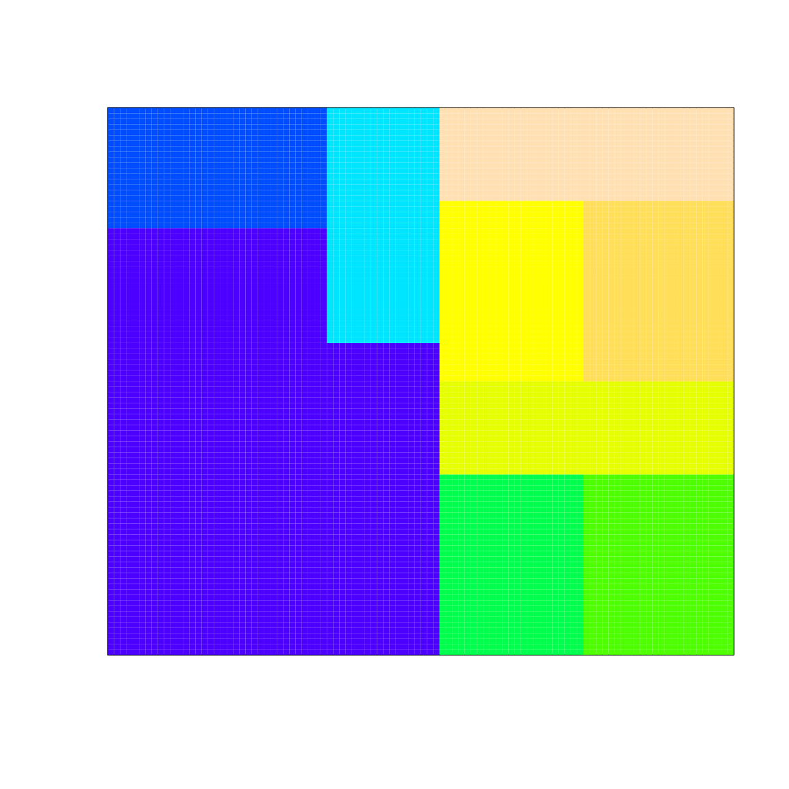
Default position of land ownership by farmers.
We can change the ownership of cells by manipulating
sim_old$LAND[,,3]. First we initialise a new
sim_old below.
sim_old  <- gmse_apply(get_res = "Full", remove_pr = 0.122, lambda = 0.275,
                       res_death_K = 93870, RESOURCE_ini = 35000,
                       manage_target = 70000, res_death_type = 3,
                       manager_budget = 10000, user_budget = 10000,
                       public_land = 0.4, stakeholders = 8, res_consume = 0.02,
                       res_birth_K = 200000, land_ownership = TRUE,
                       observe_type = 3, agent_view = 1, converge_crit = 0.01,
                       ga_mingen = 200);
Because we have not specified landscape dimensions in the above, the landscape reverts to the default size of 100 by 100 cells. We can then manually assign landscape cells to the eight farmers, whose IDs range from 2-9 (ID value 1 is the manager). Below we do this to make eight different sized farms.
sim_old$LAND[1:20,   1:20,  3] <- 2;
sim_old$LAND[1:20,  21:40,  3] <- 3;
sim_old$LAND[1:20,  41:60,  3] <- 4;
sim_old$LAND[1:20,  61:80,  3] <- 5;
sim_old$LAND[1:20,  81:100, 3] <- 6;
sim_old$LAND[21:40,  1:50,  3] <- 7;
sim_old$LAND[21:40, 51:100, 3] <- 8;
sim_old$LAND[41:60,  1:100, 3] <- 9;
sim_old$LAND[61:100, 1:100, 3] <- 1; # Public land
image(x = sim_old$LAND[,,3], col = topo.colors(9), xaxt = "n", yaxt = "n");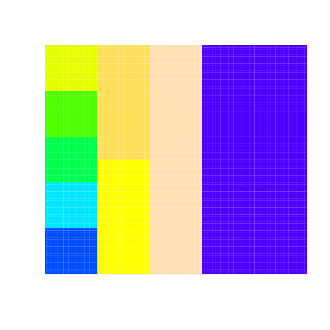
Land ownership by farmers as customised in gmse_apply.
The above image shows the modified landscape stored in
sim_old, which can now be incorporated into simulations
using gmse_apply. We can think of all the plots on the left
side of the landscape as farms of various sizes, while the blue area of
the landscape on the right is public land.
2. Parameterisation of individual user budgets
Perhaps we want to assume that farmers have different baseline
budgets, which are correlated in some way to the number of landscape
cells that they own. Custom user baseline budgets can be set by
manipulating sim_old$AGENTS, column 17 of which holds the
budget for each user. Agent IDs (as stored on the landscape above)
correspond to rows of sim_old$AGENTS, so individual
baseline budgets can be directly input as desired. We can do this
manually (e.g., sim_old$AGENTS[2, 17] <- 4000), or,
alternatively, if farmer budget positively correlates to landscape
owned, we can use a loop to input values as below.
for(ID in 2:9){
    cells_owned            <- sum(sim_old$LAND[,,3] == ID);
    sim_old$AGENTS[ID, 17] <- 10 * cells_owned;
}
The number of cells owned by the manager (1) and each farmer (2-8) is therefore listed in the table below.
| ID | 1 | 2 | 3 | 4 | 5 | 6 | 7 | 8 | 9 |
| Budget | 10000 | 4000 | 4000 | 4000 | 4000 | 4000 | 10000 | 10000 | 20000 |
As with sim_old$LAND values, changes to
sim_old$AGENTS will be retained in simulations looped
through gmse_apply.
3. Density-dependent movement of resources
Lastly, we consider a more nuanced change to simulations, in which
the rules for movement of resources are modified to account for
density-dependence. Assume that geese tend to avoid aggregating, such
that if a goose is located on the same cell as too many other geese,
then it will move at the start of a time step. Programming this movement
rule can be accomplished by creating a new function to apply to the
resource data array sim_old$resource_array. Below, a custom
function is defined that causes a goose to move up to 5 cells in any
direction if it finds itself on a cell with more than 10 other geese. As
with default GMSE simulations, movement is based on a torus landscape
(where no landscape edge exists, so that if resources move off of one
side of the landscape they appear on the opposite side). We will use
this custom function to modify sim_old$resource_array prior
to running gmse_apply, thereby modelling a custom-built
process affecting resource distribution that is integrated into
GMSE.
avoid_aggregation <- function(sim_resource_array, land_dim_1 = 100,
                              land_dim_2 = 100){
    goose_number <- dim(sim_resource_array)[1]  # How many geese are there?
    for(goose in 1:goose_number){               # Loop through all rows of geese
        x_loc  <- sim_resource_array[goose, 5];
        y_loc  <- sim_resource_array[goose, 6];
        shared <- sum( sim_resource_array[,5] == x_loc &
                       sim_resource_array[,6] == y_loc);
        if(shared > 10){
            new_x <- x_loc + sample(x = -5:5, size = 1);
            new_y <- y_loc + sample(x = -5:5, size = 1);
            if(new_x < 0){ # The 'if' statements below apply the torus
                new_x <- land_dim_1 + new_x;
            }
            if(new_x >= land_dim_1){
                new_x <- new_x - land_dim_1;
            }
            if(new_y < 0){
                new_y <- land_dim_2 + new_x;
            }
            if(new_y >= land_dim_2){
                new_y <- new_y - land_dim_2;
            }
            sim_resource_array[goose, 5] <- new_x;
            sim_resource_array[goose, 6] <- new_y;
        }
    }
    return(sim_resource_array);
}
With the above function written, we can apply the new movement rule along with our custom farm placement and custom farmer budgets to the simulation of goose population dynamics.
Simulation with custom farms, budgets, and goose movement
Below shows an example of gmse_apply with custom
landscapes, farmer budgets, and density-dependent goose movement
rules.
# First initialise a simulation
sim_old  <- gmse_apply(get_res = "Full", remove_pr = 0.122, lambda = 0.275,
                       res_death_K = 93870, RESOURCE_ini = 35000,
                       manage_target = 70000, res_death_type = 3,
                       manager_budget = 10000, user_budget = 10000,
                       public_land = 0.4, stakeholders = 8, res_consume = 0.02,
                       res_birth_K = 200000, land_ownership = TRUE,
                       observe_type = 3, agent_view = 1, converge_crit = 0.01,
                       ga_mingen = 200, res_move_type = 0);
# By setting `res_move_type = 0`, no resource movement will occur in gmse_apply
# Adjust the landscape ownership below
sim_old$LAND[1:20,   1:20,  3] <- 2;
sim_old$LAND[1:20,  21:40,  3] <- 3;
sim_old$LAND[1:20,  41:60,  3] <- 4;
sim_old$LAND[1:20,  61:80,  3] <- 5;
sim_old$LAND[1:20,  81:100, 3] <- 6;
sim_old$LAND[21:40,  1:50,  3] <- 7;
sim_old$LAND[21:40, 51:100, 3] <- 8;
sim_old$LAND[41:60,  1:100, 3] <- 9;
sim_old$LAND[61:100, 1:100, 3] <- 1;
# Change the budgets of each farmer based on the land they own
for(ID in 2:9){
    cells_owned            <- sum(sim_old$LAND[,,3] == ID);
    sim_old$AGENTS[ID, 17] <- 10 * cells_owned;
}
# Begin simulating time steps for the system
sim_sum_2 <- matrix(data = NA, nrow = 30, ncol = 5);
for(time_step in 1:30){
    # Apply the new movement rules at the beginning of the loop
    sim_old$resource_array  <- avoid_aggregation(sim_resource_array =
                                                     sim_old$resource_array);
    # Next, move on to simulate (old_list remembers that res_move_type = 0)
    sim_new                 <- gmse_apply(get_res = "Full", old_list = sim_old);
    sim_sum_2[time_step, 1] <- time_step;
    sim_sum_2[time_step, 2] <- sim_new$basic_output$resource_results[1];
    sim_sum_2[time_step, 3] <- sim_new$basic_output$observation_results[1];
    sim_sum_2[time_step, 4] <- sim_new$basic_output$manager_results[3];
    sim_sum_2[time_step, 5] <- sum(sim_new$basic_output$user_results[,3]);
    sim_old                 <- sim_new;
}
colnames(sim_sum_2) <- c("Time", "Pop_size", "Pop_est", "Cull_cost",
                         "Cull_count");
print(sim_sum_2);
## Time Pop_size Pop_est Cull_cost Cull_count
## [1,] 1 33435 33435 1008 52
## [2,] 2 33562 33562 1010 52
## [3,] 3 34467 34467 998 60
## [4,] 4 35898 35898 1002 52
## [5,] 5 41222 41222 1010 52
## [6,] 6 43201 43201 992 60
## [7,] 7 45494 45494 1010 52
## [8,] 8 48070 48070 999 60
## [9,] 9 51173 51173 1006 52
## [10,] 10 54558 54558 1008 52
## [11,] 11 58090 58090 1010 52
## [12,] 12 61635 61635 1000 60
## [13,] 13 65631 65631 1005 52
## [14,] 14 70030 70030 1009 52
## [15,] 15 74541 74541 14 4099
## [16,] 16 75133 75133 12 4646
## [17,] 17 75393 75393 12 4636
## [18,] 18 75571 75571 11 4983
## [19,] 19 75425 75425 12 4666
## [20,] 20 75491 75491 12 4658
## [21,] 21 75854 75854 12 4650
## [22,] 22 76014 76014 11 5004
## [23,] 23 75801 75801 11 4996
## [24,] 24 75521 75521 11 4997
## [25,] 25 75064 75064 12 4680
## [26,] 26 75100 75100 13 4379
## [27,] 27 75912 75912 11 5032
## [28,] 28 76896 76896 10 5404
## [29,] 29 77964 77964 10 5382
## [30,] 30 79982 79982 10 5476Conclusions
In this example, we showed how the built-in resource, observation,
manager, and user sub-models can be customised by manipulating the data
within the data structures that they use. The goal was to show how
software users can work with these existing sub-models and data
structures to customise GMSE simulations. Readers seeking even greater
flexibility (e.g., replacing an entire built-in sub-model with a custom
sub-model) should refer to Use of the gmse_apply
function that introduces gmse_apply more generally.
Future versions of GMSE are likely to expand on the built-in options
available for simulation; requests for such expansions, or
contributions, can be submitted to GitHub.