Fisheries example integrating FLR
GMSE: an R package for generalised management strategy evaluation (Supporting Information 5)
A. Bradley Duthie¹³, Jeremy J. Cusack¹, Isabel L.
Jones¹, Jeroen Minderman¹,
Erlend B. Nilsen², Rocío A. Pozo¹, O. Sarobidy Rakotonarivo¹,
Bram Van Moorter², and Nils Bunnefeld¹
Erlend B. Nilsen², Rocío A. Pozo¹, O. Sarobidy Rakotonarivo¹,
Bram Van Moorter², and Nils Bunnefeld¹
[1] Biological and Environmental Sciences, University of Stirling, Stirling, UK [2] Norwegian Institute for Nature Research, Trondheim, Norway [3] alexander.duthie@stir.ac.uk
Source:vignettes/SI5.Rmd
SI5.RmdIntegration and simulation with fisheries
Early development of management strategy evaluation (MSE) models originated in fisheries (Polacheck et al. 1999; Smith, Sainsbury, and Stevens 1999; Sainsbury, Punt, and Smith 2000). Consequently, fisheries-focused software for MSE has been extensively developed, including R libraries that focus on the management of species of exceptional interest, such as the Atlantic Bluefin Tuna (Thunnus thynnus) [ABFTMSE; Carruthers and Butterworth (2018a); Carruthers and Butterworth (2018b)], and Indian Ocean Bigeye (T. obesus) and Yellowfin (T. albacares) Tuna [MSE-IO-BET-YFT; Kolody and Jumppanen (2016)]. The largest of all such libraries is the Fisheries Library in R (FLR), which includes an extensive collection of tools targeted for fisheries science. The FLR library has been used in over a hundred publications (recent publications include Jardim et al. 2018; Mackinson et al. 2018; Utizi et al. 2018), and includes an MSE framework for evaluating different harvest control rules.
As part of the ConFooBio
project, a central focus of GMSE is on simulating the management of
animal populations of conservation interest, with a particular emphasis
on understanding conservation conflict; further development of GMSE is
expected to continue with this as a priority, further building upon the
decision-making algorithms of managers and users to better understand
how conflict arises and can be managed and mitigated. Hence, GMSE is not
intended as a substitute for packages such as FLR, but the integration of these
packages with GMSE could make use of GSME’s current and future
simulation capabilities, and particularly the genetic
algorithm. Such integration might be possible using the
gmse_apply function, which allows for custom defined sub-models to be used within the GMSE
framework, and with default GMSE sub-models. Hence, GMSE might be
especially useful for modelling the management of fisheries under
conditions of increasing competing stakeholder demands and conflicts. We
do not attempt such an ambitious project here, but instead show how such
a project could be developed through integration of FLR and
gmse_apply.
Here we follow a Modelling
Stock-Recruitment with FLSR example, then integrate this example
with gmse_apply to explore the behaviour of a number of
simulated fishers who are goal-driven to maximise their own harvest and
a manager that aims to keep the fish stocks at a predefined target
level. The core concept in GMSE is that manager can only incentivise
fishers to harvest less or more by varying the cost of fishing (through
e.g. taxes) given a set manager budget; please note that the manager
cannot force the fisher to follow any policy. Based on the cost of
fishing, the fisher can then given their own budget decide whether to
invest in fishing or keep the budget. This concepts represents a
nartural resource managmeent and conservation conflict, where one party
aims to maximise their livelihood (fisher) and the other aims to keep a
population at a sustainable level and prevent it from going extinct.
Importantly, the manager does not have full control over fishers but can
set policies to incentivise sustainable behaviour. We emphasise that
this example is provided only as demonstration of how GMSE can
potentially be integrated with already developed fisheries models, and
is not intended to make recommendations for management in any
population.
Integrating with the Fisheries Library in R (FLR)
The FLR toolset includes a series of packages,
with several tutorials for using
them. For simplicity, we focus on a
model of stock recruitment to be used as the population model in
gmse_apply. This population model will use sample data and
one of the many available stock-recruitment models available in FLR, and
a custom function will be written to return a single value for stock
recruitment. Currently, gmse_apply requires that sub-models
return subfunction results either as scalar values or data frames that
are structured in the same way as GMSE sub-models.
But interpretation of scalar values is left up to the user (e.g.,
population model results could be interpreted as abundance or biomass;
manager policy could be interpreted as cost of harvesting or as total
allowable catch). For simplicity, the observation (i.e., estimation)
model will be the stock reported from the population model with error.
The manager and user models, however, will employ the full power of the
default GMSE functions to simulate management and user actions. We first
show how a custom function can be made that applies the FLR toolset to a
population model.
Modelling stock-recruitment for the population model
Here we closely follow a
tutorial from the FLR project. To build the stock-recruitment model,
the FLCore package is needed (Kell et al. 2007).
We also include the ggplotFL package for plotting.
install.packages("FLCore", repos="http://flr-project.org/R");
install.packages("ggplotFL", repos="http://flr-project.org/R")
To start, we need to read in the FLCore,
ggplotFL and GMSE libraries.
## Loading required package: lattice## Loading required package: iterators## FLCore (Version 2.6.18, packaged: 2021-10-28 15:07:14 UTC)## Loading required package: ggplot2##
## Attaching package: 'ggplot2'## The following object is masked from 'package:FLCore':
##
## %+%For a simplified example in GMSE, we will simulate the process of
stock recruitment over multiple time steps using an example
stock-recruitment model. The stock-recruitment model describes the
relationship between stock-recruitment and spawning stock biomass. The
sample that we will work from is a recreation of the North Sea Herring
(nsher) dataset available in the FLCore
package (Kell et al. 2007). This data set
includes recruitment and spawning stock biomass data between 1960 and
2004. First, we initialise an empty FLSR object and read in
the recreated herring data files from GMSE, which contains recruitment
(rec.n) and spawning stock biomass (ssb.n)
newFL   <- FLSR(); # Initialises the empty FLSR object
data(nsher_data);  # Called from GMSE library (not from FLCore)
The recruitment (rec.n) and spawning stock biomass
(ssb.n) data need to be in the form of a vector, array,
matrix to use them with FLQuant. We will convert
rec.n and ssb.n into matrices.
We can then construct two FLQuant objects, specifying
the relevant years and units.
Frec.m <- FLQuant(rec.m, dimnames=list(age=1, year = 1960:2004));
Fssb.m <- FLQuant(ssb.m, dimnames=list(age=1, year = 1960:2004));
Frec.m@units <- "10^3";
Fssb.m@units <- "t*10^3";We then place the recruitment and spawning stock biomass data into
the FLSR object that we created.
The FLCore package offers several stock-recruitment
models. Here we use a Ricker model of stock recruitment (Ricker
1954), and insert this model into the FLSR
object below.
Parameters for the Ricker stock-recruitment model can be estimated with maximum likelihood.
newFL <- fmle(newFL);Diagnostic plots, identical to those of the modelling
stock-recruitment tutorial for the nsher_ri example,
are shown below in Figure 1. We note that these plots are made using the
FLCore and ggplotFL packages, and are not
produced by, nor available in, the GMSE package.
plot(newFL, cex = 0.7);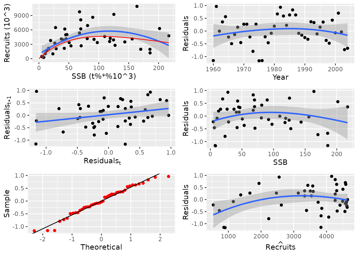
Output of the FLR plot function for an example Ricker model of stock recruitment on North Sea Herring data.
We now have a working example of a stock-recruitment model, but for
our integration with gmse_apply, we will want a function
that automates the above to simulate the process of updating the
stock-recruitment model. We do this using the custom function created
below.
update_SR_model <- function(rec_m, ssb_m, years){
Frec_m <- FLQuant(rec_m, dimnames=list(age = 1, year = years));
Fssb_m <- FLQuant(ssb_m, dimnames=list(age = 1, year = years));
Frec_m@units <- "10^3";
Fssb_m@units <- "t*10^3";
rec(newFL) <- Frec.m;
ssb(newFL) <- Fssb.m;
range(newFL) <- c(0, years[1], 0, years[length(years)]);
model(newFL) <- ricker();
newFL <- fmle(newFL);
return(newFL);
}The above function will be used within another custom function to predict the next time step of recruitment.
predict_recruitment <- function(rec_m, ssb_m, years, new_ssb){
newFL <- update_SR_model(rec_m, ssb_m, years);
a <- params(newFL)[[1]] # Extract 'a' parameter of the Ricker model
b <- params(newFL)[[2]] # Extract 'b' parameter of the Ricker model
rec <- a * new_ssb * exp(-b * new_ssb); # Predict the new recruitment
return(rec)
}In gmse_apply, we will use the
predict_recruitment function above as the resource (i.e.,
operational) model. The new_ssb reads in the new spawning
stock biomass, which will be calculated from the built-in GMSE
user model.
Integrating predict_recruitment with
gmse_apply
The FLR project includes
libraries that can be used to perform
a management strategy evaluation (MSE) under fisheries-focused
observation, manager, and user models. We will not recreate this
approach, or integrate any other sub-models into GMSE as was done
for the population model above, although such integration of sub-models
should be possible using similar techniques. Our goal here is to instead
show how the predict_recruitment model created above can be
integrated with gmse_apply, which can then make use of the
genetic algorithm to predict the fishers’ behaviour.
We will use a custom observation model, which will simply estimate recruitment with some fixed error.
obs_ssb <- function(resource_vector){
obs_err <- rnorm(n = 1, mean = 0, sd = 100);
the_obs <- resource_vector + obs_err;
return(the_obs);
}Hence, we can now feed the data from rec.m and
ssb.m through predict_recruitment, which will
return a value for new recruitment, and this new value can in turn be
fed into obs_ssb to predict recruitment with some error. We
also need a new spawning stock biomass new_ssb, which we
can just initialise with the biomass from the last year in
ssb.m
ssb_ini <- ssb.m[length(ssb.m)];
new_rec <- predict_recruitment(rec_m = rec.m, ssb_m = ssb.m, years = 1960:2004,
new_ssb = ssb_ini);
obs_rec <- obs_ssb(new_rec);An initial run of these models gives values of 3835.21 for
new_rec and 3872.78 for obs_rec. We are now
ready to use the built-in manager and user sub-models in
gmse_apply. We will assume that managers attempt to keep a
recruitment of 5000, and that there are 10 independent fishers who
attempt to maximise their catch. We assign a user budget of
manager_budget = 10000, and all other values are set to
GMSE defaults. In the built-in GMSE functions, the manager will use the
estimate of recruitment based on obs_rec and use it to set
the cost of harvesting (culling in GMSE).
yrspan <- 1960:2004;
rec.m        <- as.matrix(rec.n);
ssb.m        <- as.matrix(ssb.n);
sim <- gmse_apply(res_mod = predict_recruitment, obs_mod = obs_ssb,
rec_m = rec.m, ssb_m = ssb.m, years = yrspan,
new_ssb = ssb_ini, manage_target = 5000, stakeholders = 10,
manager_budget = 10000);
print(sim);## $resource_results
## [1] 3835
##
## $observation_results
## [1] 3946.299
##
## $manager_results
## resource_type scaring culling castration feeding help_offspring
## policy_1 1 NA 458 NA NA NA
##
## $user_results
## resource_type scaring culling castration feeding help_offspring
## Manager 1 NA 0 NA NA NA
## user_1 1 NA 2 NA NA NA
## user_2 1 NA 2 NA NA NA
## user_3 1 NA 2 NA NA NA
## user_4 1 NA 2 NA NA NA
## user_5 1 NA 2 NA NA NA
## user_6 1 NA 2 NA NA NA
## user_7 1 NA 2 NA NA NA
## user_8 1 NA 2 NA NA NA
## user_9 1 NA 2 NA NA NA
## user_10 1 NA 2 NA NA NA
## tend_crops kill_crops
## Manager NA NA
## user_1 NA NA
## user_2 NA NA
## user_3 NA NA
## user_4 NA NA
## user_5 NA NA
## user_6 NA NA
## user_7 NA NA
## user_8 NA NA
## user_9 NA NA
## user_10 NA NAThe resource and observation results above are interpreted in terms
of recruitment, while the manager results are interpreted in terms of
the cost of harvesting a unit of spawning stock biomass and the user
results are interpreted in terms of how much biomass was harvested. Note
in the run of gmse_apply that the arguments for our custom
resource and observation models (predict_recruitment and
obs_ssb, respectively) are read directly in as arguments of
gmse_apply itself. The gmse_apply function
will figure out which subfunctions custom arguments should go to, then
update these arguments as needed over the course of a single run of
gmse_apply.
Simulation with gmse_apply over multiple time
steps
We are now ready to loop the gmse_apply function over
multiple time steps. To do this, we will update the rec.m
and ssb.m matrices after each time step, simulating 20
years into the future. The population model
predict_recruitment will use these data to dynamically
update parameters of the Ricker model, as might occur in an empirical
fishery that is being monitored. We will use the results from the
observation model to update recruitment for the new year in
rec.m. For simplicity, spawning stock biomass prior to
harvest will be randomly sampled from a value in the last 10 years
(i.e., from ssb.m between 1994 and 2004), but more
realistic models could relate this spawning stock biomass to recruitment
and environmental variables from a previous year; spawning stock biomass
will be decreased after harvest based on user actions. The GMSE
initialisation and simulation is below.
# This code initialises the simulation -----------------------------------------
yrspan       <- 1960:2004;
rec.m        <- as.matrix(rec.n);
ssb.m        <- as.matrix(ssb.n);
ssb_ini      <- ssb.m[length(ssb.m)];
sim_old      <- gmse_apply(res_mod = predict_recruitment, obs_mod = obs_ssb,
                           rec_m = rec.m, ssb_m = ssb.m, years = yrspan,
                           new_ssb = ssb_ini, manage_target = 3500,
                           stakeholders = 10, manager_budget = 10000,
                           get_res = "Full");
# The code below simulates 20 time steps ---------------------------------------
sim_sum  <- matrix(data = NA, nrow = 20, ncol = 6); # Hold results here
for(time_step in 1:20){
    # Update the relevant parameter values as necessary -----------------------
    rand_ssb        <- sample(x = ssb.m[35:45], size = 1);
    harvest         <- sum(sim_old$basic_output$user_results[,3]);
    new_rec_m       <- c(sim_old$rec_m, sim_old$observation_vector);
    new_ssb_m       <- c(sim_old$ssb_m, rand_ssb - harvest);
    sim_old$rec_m   <- matrix(data = new_rec_m, nrow = 1);
    sim_old$ssb_m   <- matrix(data = new_ssb_m, nrow = 1);
    sim_old$years   <- c(sim_old$years, time_step + 2004);
    sim_old$new_ssb <- sim_old$ssb_m[length(sim_old$ssb_m)];
    # Run a new simulation in the loop: custom functions are always specified -
    sim_new  <- gmse_apply(get_res = "Full", old_list = sim_old,
                           res_mod = predict_recruitment, obs_mod = obs_ssb);
    # Record the results in sim_sum -------------------------------------------
    sim_sum[time_step, 1] <- time_step + 2004;
    sim_sum[time_step, 2] <- sim_new$basic_output$resource_results[1];
    sim_sum[time_step, 3] <- sim_new$basic_output$observation_results[1];
    sim_sum[time_step, 4] <- sim_new$basic_output$manager_results[3];
    sim_sum[time_step, 5] <- harvest;
    sim_sum[time_step, 6] <- sim_new$new_ssb;
    # Redefine the old list --------------------------------------------------
    sim_old               <- sim_new;
}
colnames(sim_sum) <- c("Year", "Recruitment", "Recruit_estim", "Harvest_cost",
                         "Harvested", "SSB");
print(sim_sum);
## Year Recruitment Recruit_estim Harvest_cost Harvested SSB
## [1,] 2005 3747 3843.480 222 20 50.6639
## [2,] 2006 4547 4465.442 230 40 85.2627
## [3,] 2007 4390 4406.651 240 40 145.5799
## [4,] 2008 1146 1136.166 693 40 10.6133
## [5,] 2009 4082 4106.639 217 10 60.6639
## [6,] 2010 4541 4568.789 221 40 130.1926
## [7,] 2011 3310 3192.144 700 40 40.7603
## [8,] 2012 4082 4086.803 217 10 60.6639
## [9,] 2013 4390 4385.348 226 40 145.5799
## [10,] 2014 2739 2662.746 684 40 30.6639
## [11,] 2015 3303 3290.138 869 10 40.6133
## [12,] 2016 3035 3061.967 968 10 35.5913
## [13,] 2017 3303 3376.865 1008 10 40.6133
## [14,] 2018 3855 3798.617 250 0 53.5966
## [15,] 2019 4541 4635.799 231 40 130.1926
## [16,] 2020 3310 3318.888 689 40 40.7603
## [17,] 2021 4082 4092.835 235 10 60.6639
## [18,] 2022 633 614.248 692 40 5.5913
## [19,] 2023 3988 3745.669 235 10 175.5799
## [20,] 2024 4627 4666.104 228 40 115.9025The above output from sim_sum reports the recruitment
(resource or operational model), recruitment estimate (observation error
model), management set harvest cost (harvest control model), user
harvested numbers (implementation model) and spawning stock biomass
(SSB) simulation results. This example simulation demonstrates the
ability of GMSE to integrate with fisheries libraries such as FLR through
gmse_apply. In addition to being a useful wrapping function
for MSE sub-models, gmse_apply can therefore be used to
take advantage of the genetic algorithm in the GMSE default manager and
user models. This flexibility will be retained in future versions of
gmse_apply, allowing custom resource and observation models
that are built for specific systems to be integrated with an
increasingly complex genetic algorithm simulating various aspects of
human decision-making.
Conclusions
GMSE is a general, flexible, tool for simulating the management of resources under situations of uncertainty and conflict. Management Strategy Evaluation (Bunnefeld et al. 2011; Punt et al. 2016), the framework upon which GMSE is based, had its origin in fisheries management (Polacheck et al. 1999; Smith, Sainsbury, and Stevens 1999; Sainsbury, Punt, and Smith 2000), and here we showed one example of how GMSE could be integrated with the core package of the Fisheries Library in R.
Future versions of GMSE will continue to be open-source and developed
to avoid unecessary dependencies (GMSE requires only base R, plus three
shiny packages for running gmse_gui). Key goals including
(1) providing highly general and useful default resource,
observation, manager, and user
sub-models for a variety of MSE modelling tasks, (2) keeping these
sub-models highly modular so that they can be developed in isolation
given standardised data structures, and (3) allowing these modular
sub-models to be integrated with custom defined sub-models as flexibly
as possible using gmse_apply. Contributions in line with
these goals, and suggestions for new features, can be made on GitHub.