Default GMSE data structures
GMSE: an R package for generalised management strategy evaluation (Supporting Information 7)
A. Bradley Duthie¹³, Jeremy J. Cusack¹, Isabel L.
Jones¹, Jeroen Minderman¹,
Erlend B. Nilsen², Rocío A. Pozo¹, O. Sarobidy Rakotonarivo¹,
Bram Van Moorter², and Nils Bunnefeld¹
Erlend B. Nilsen², Rocío A. Pozo¹, O. Sarobidy Rakotonarivo¹,
Bram Van Moorter², and Nils Bunnefeld¹
[1] Biological and Environmental Sciences, University of Stirling, Stirling, UK [2] Norwegian Institute for Nature Research, Trondheim, Norway [3] alexander.duthie@stir.ac.uk
Source:vignettes/SI7.Rmd
SI7.RmdThe most important (default) GMSE data structures
The default sub-models of GMSE (resource,
observation, manager, and user)
use a small number of default data structures to hold the information
needed in simulations. While these default sub-models do not necessarily
need to be used in every run in GMSE (see use of
gmse_apply), they will be used in any run of the
gmse function, and in any call of the
gmse_apply function that does not run with entirely custom
sub-models. Simulation and model inference do not require an
understanding of the default data structures, but such an understanding
can be especially useful when running gmse_apply if there
is a need to extract uncommonly used information, change key simulated
values (e.g., landscape properties, agent budgets, or resource movement
rules, as in Advanced case study options), or
build custom individual-based sub-models. Here we provide a brief
explanation of the following key data structures (each name below is
listed as it is named in the output gmse_apply when
get_res = "Full").
AGENTS-
resource_array(orRESOURCES) -
observation_array(orOBSERVATION) -
manager_array(orCOST) -
user_array(orACTION) LAND
Note that these are not the only data structures used in GMSE, but
they are the only ones that can be easily modified in GMSE (see, e.g.,
Advanced case study options), so they are the
ones that we focus on here. Additionally, any custom subfunction that
returns an array rather than a single value should adhere to the same
structure as these defaults if any default GMSE functions are to be used
in gmse_apply. We can investigate each data structure by
running a single simulation of gmse_apply.
sim <- gmse_apply(get_res = "Full");The full list output of sim holds each structure by name
(in the case where two names are used, e.g., resource_array
and RESOURCES, both are identical, but the lower case
resource_array takes precedence in case of a change). Each
data structure can be examined, changed, and incorporated into a new
simulation (e.g.,
new_sim <- gmse_apply(old_list = sim)).
1. AGENTS
The AGENTS data structure is a two dimensional array
with a fixed number of 27 columns and a number of rows that is always
equal to the sum of the number of manager and users (i.e., each row is
an individual agent).
print(sim$AGENTS);## [,1] [,2] [,3] [,4] [,5] [,6] [,7] [,8] [,9] [,10] [,11] [,12] [,13] [,14]
## [1,] 1 0 0 0 98 37 50 0 10 0 48 0 0 10000
## [2,] 2 1 0 0 68 8 50 0 10 0 0 0 0 0
## [3,] 3 1 0 0 70 24 50 0 10 0 0 0 0 0
## [4,] 4 1 0 0 67 57 50 0 10 0 0 0 0 0
## [5,] 5 1 0 0 67 20 50 0 10 0 0 0 0 0
## [,15] [,16] [,17] [,18] [,19] [,20] [,21] [,22] [,23] [,24] [,25] [,26]
## [1,] 0 9512.125 1000 0 -1.17 0 0 0 0 0 0 0
## [2,] 0 0.000 1000 0 -1.30 0 0 0 0 0 0 0
## [3,] 0 0.000 1000 0 -1.30 0 0 0 0 0 0 0
## [4,] 0 0.000 1000 0 -1.30 0 0 0 0 0 0 0
## [5,] 0 0.000 1000 0 -1.30 0 0 0 0 0 0 0
## [,27]
## [1,] 0
## [2,] 0
## [3,] 0
## [4,] 0
## [5,] 0In the default case above, there are five agents (one manager and four users), each represented by a unique row. Columns in the array represent the agent traits listed below.
- ID (each agent gets a unique number)
- Type 1 (0 indicates the manager; 1 indicates users)
- Type 2 (currently unused)
- Type 3 (currently unused)
- x-location on the landscape (typically ignored)
- y-location on the landscape (typically ignored)
- Movement distance (typically ignored)
- Time parameter (typically ignored)
- Distance of vision (currently used only for managers)
- Error parameter (currently unused)
- Resource marking parameter (currently used only for managers)
- Resource tally parameter (currently used only for managers)
- How many resources an agent has in view (unused)
- Total number of cells owned by an agent
- Unused column
- Yield from owned land (zero for users when default
land_ownership = FALSE) - Agent’s baseline budget
- Agent’s perception of the efficacy of scaring one resource
- Agent’s perception of the efficacy of culling one resource
- Agent’s perception of the efficacy of castrating one resource
- Agent’s perception of the efficacy of feeding one resource
- Agent’s perception of the efficacy of helping offspring of one resource
- Agent’s perception of the efficacy of tending the crop on one landscape cell
- Agent’s perception of the efficacy of killing the crop on one landscape cell
- Increment added to the manager’s (row 1) baseline budget caused by a budget bonus
- Increment added to an agent’s budget caused by yield
- Unused column
Note that for the perceptions of the efficacy of different actions (columns 18-24), this relates to whatever it is that the agents are acting upon. For example, for columns 18-22, actions are on the resources, so if an agent’s perception of the efficacy of scaring is -1, this means that they believe that scaring a resource will decrease the number of resources affecting them by 1 (lower default values for landowners are caused based on the probability of a scared resource landing on a different cell owned by the same agent). For columns 23-24, actions are on the landscape, so if an agent tends the crop on one landscape cell, this value defines an agent’s perception of how much yield on that cell will increase.
It is obvious from the above list that several columns represent
traits that are either typically ignored or currently not in use. This
is intended to allow for easier future development of default model
options and potential customisation of sub-models in
gmse_apply. We anticipate that future versions of GMSE will
contain multiple user types with unique traits and among-user
interactions.
2. resource_array
The resource_array (also accessible as
RESOURCES) is a two dimensional array with a fixed number
of 22 columns and a number of rows that is always equal to the total
number of resources (each row is an individual resource). In the above
simulation, sim$resource_array includes 1050 rows, so we
only print out the first eight for illustration.
print(sim$resource_array[1:8,]);## [,1] [,2] [,3] [,4] [,5] [,6] [,7] [,8] [,9] [,10] [,11] [,12] [,13] [,14]
## [1,] 1 1 0 0 34 70 20 1 0 0.3 0 4 0 0
## [2,] 2 1 0 0 12 2 20 1 0 0.3 1 5 0 0
## [3,] 3 1 0 0 60 94 20 1 0 0.3 0 2 0 0
## [4,] 4 1 0 0 56 23 20 1 0 0.3 0 3 0 0
## [5,] 5 1 0 0 51 66 20 1 0 0.3 2 5 0 0
## [6,] 6 1 0 0 14 9 20 1 0 0.3 0 3 0 0
## [7,] 7 1 0 0 80 56 20 1 0 0.3 0 2 0 0
## [8,] 8 1 0 0 50 68 20 1 0 0.3 0 5 0 0
## [,15] [,16] [,17] [,18] [,19] [,20] [,21] [,22]
## [1,] 0.5 0 0 0 0 0 0 1
## [2,] 0.5 0 0 0 0 0 0 1
## [3,] 0.5 0 4 0 0 0 0 1
## [4,] 0.5 0 0 0 0 0 0 1
## [5,] 0.5 0 0 0 0 0 0 1
## [6,] 0.5 0 0 0 0 0 0 1
## [7,] 0.5 0 0 0 0 0 0 1
## [8,] 0.5 0 0 0 0 0 0 1Columns in the resource array represent the individual resource traits listed below.
- ID (each resource gets a unique number)
- Type 1 (currently all resources are of type 1)
- Type 2 (currently unused)
- Type 3 (currently unused)
- x-location on the landscape
- y-location on the landscape
- Movement distance
- Time parameter (typically ignored)
- Density-independent removal (i.e., death) probability
- Growth (i.e., birth) probability
- Offspring produced
- Age (initial resources are given a random age between 1 and the maximum age sampled from a uniform distribution; offspring always start at age zero in their time step of birth)
- Marking indicator (used in the observation function)
- Tallying indicator (used in the observation function)
- Proportion of a landscape cell the resource consumes in a time step
- Has the resource been scared by an agent?
- Has the resource been culled by an agent?
- Has the resource been castrated by an agent?
- Has the resource’s growth rate been increased by an agent?
- Has the resource’s offspring production been increased by an agent?
- How much yield has the resource consumed?
- How many times can the resource consume yield in one time step?
In the case of columns 16-20, the value is either zero (if no action has occurred), or some positive integer that matches the ID of the agent that has performed the act (e.g., if column 17 equals 3, then that means that the agent with ID = 3 culled the resource in the corresponding row; where more than one agent’s action is possible per time step – as in scaring – the integer reflects the most recently acting agent). We anticipate that future versions of gmse will contain multiple resource types, and might add columns to include additional resource traits.
3. observation_array
The observation_array (also accessible as
OBSERVATION) is a two dimensional array, the number of rows
and columns of which depend on the type of observation being made (i.e.,
observe_type, which can take integer values from 0-3; see
the GMSE reference
manual for more information about built-in observation types that
are available in GMSE). The first 20 columns of
observation_array contain the same individual resource
traits as in resource_array, while any additional columns
provide information about how and when a resource was observed. The
number of rows in observation_array is always equal to or
less than that of resource_array; each resource that is
observed at least once is placed into one unique row, while unobserved
resources are not included as rows in the
observation_array. In sim, there are 48 rows,
meaning that 1002 resources were not observed at all in this time step.
Below, we print out the first eight rows of the observation array.
print(sim$observation_array[1:8,]);## [,1] [,2] [,3] [,4] [,5] [,6] [,7] [,8] [,9] [,10] [,11] [,12] [,13] [,14]
## [1,] 65 1 0 0 5 36 20 1 0 0.3 0 4 1 0
## [2,] 137 1 0 0 4 41 20 1 0 0.3 0 3 1 0
## [3,] 146 1 0 0 96 27 20 1 0 0.3 1 2 1 0
## [4,] 201 1 0 0 8 30 20 1 0 0.3 0 4 1 0
## [5,] 207 1 0 0 89 46 20 1 0 0.3 0 2 1 0
## [6,] 318 1 0 0 90 43 20 1 0 0.3 0 4 1 0
## [7,] 387 1 0 0 88 47 20 1 0 0.3 1 2 1 0
## [8,] 393 1 0 0 91 41 20 1 0 0.3 0 5 1 0
## [,15] [,16] [,17] [,18] [,19] [,20] [,21] [,22] [,23] [,24]
## [1,] 0.5 0 0 0 0 0 0 1 0 1
## [2,] 0.5 0 0 0 0 0 0 1 0 1
## [3,] 0.5 0 0 0 0 0 0 1 0 1
## [4,] 0.5 0 0 0 0 0 0 1 0 1
## [5,] 0.5 0 0 0 0 0 0 1 0 1
## [6,] 0.5 0 0 0 0 0 0 1 0 1
## [7,] 0.5 0 0 0 0 0 0 1 0 1
## [8,] 0.5 0 0 0 0 0 0 1 0 1In the case of the default parameters, the observation array has only
two additional columns; the first added column 21 is currently unused,
and all values in this column are zero. The second added column 22
contains a value of 1 confirming that the resource was observed.
Additional options will add different numbers of columns with different
values. For example, when observe_type = 0 (managers
observe all resources on a random subset of the landscape, the size of
which is determined by their distance of vision) but
times_observe > 1, managers sample more than one random
subset of the landscape. A new column is added for each sampled subset,
and a 1 is placed in the relevant column if the resource is observed
(these collected data are then used to estimate population size). An
example where times_observe = 4 is shown below.
sim_t0_4 <- gmse_apply(get_res = "Full", times_observe = 4);
print(sim_t0_4$observation_array[1:8,]);
## [,1] [,2] [,3] [,4] [,5] [,6] [,7] [,8] [,9] [,10] [,11] [,12] [,13] [,14]
## [1,] 1 1 0 0 48 72 20 1 0 0.3 0 2 1 0
## [2,] 4 1 0 0 89 94 20 1 0 0.3 0 5 1 0
## [3,] 14 1 0 0 84 97 20 1 0 0.3 0 4 1 0
## [4,] 15 1 0 0 94 5 20 1 0 0.3 0 5 1 0
## [5,] 18 1 0 0 75 29 20 1 0 0.3 0 5 1 0
## [6,] 40 1 0 0 54 64 20 1 0 0.3 0 2 1 0
## [7,] 42 1 0 0 50 66 20 1 0 0.3 1 5 1 0
## [8,] 54 1 0 0 52 77 20 1 0 0.3 0 3 1 0
## [,15] [,16] [,17] [,18] [,19] [,20] [,21] [,22] [,23] [,24] [,25] [,26]
## [1,] 0.5 0 0 0 0 0 0 1 0 0 1 0
## [2,] 0.5 0 0 0 0 0 0 1 0 1 0 0
## [3,] 0.5 0 0 0 0 0 0 1 0 1 0 0
## [4,] 0.5 0 0 0 0 0 0 1 0 1 0 0
## [5,] 0.5 0 0 0 0 0 0 1 0 0 0 0
## [6,] 0.5 0 0 0 0 0 0 1 0 0 1 0
## [7,] 0.5 0 0 0 0 0 0 1 0 0 1 0
## [8,] 0.5 0 0 0 0 0 0 1 0 0 1 0
## [,27]
## [1,] 0
## [2,] 0
## [3,] 0
## [4,] 0
## [5,] 1
## [6,] 0
## [7,] 0
## [8,] 0This process simulates the data collection of resources (and potentially resource trait measurement) as might be performed by observers within the system. It therefore takes a virtual ecologist approach; this enables the integration of theory and empirical work and can improve the mechanistic understanding of social-ecological systems (Zurell et al. 2010).
4. manager_array
For context, it might be easier to understand
manager_array after reading about user_array
below. The manager_array (also
accessible as COST) is a three dimensional array, each
layer of which corresponds to a unique agent (rows in AGENT correpond to layers in
manager_array). Hence, in the simulation output
sim$manager_array, there are 5 layers. Each layer in
manager_array has 13 columns, and a number of rows that
varies depending on the number of agents and resource types. As of GMSE
v0.4.0.7, only the first three rows are used. Two layers of
sim$manager_array are shown below, the first being that of
the manager and the second being that of the first user.
print(sim$manager_array[,,1:2]);## , , 1
##
## [,1] [,2] [,3] [,4] [,5] [,6] [,7] [,8] [,9] [,10]
## [1,] 100001 100001 100001 100001 100001 100001 100001 100001 100001 100001
## [2,] 100001 100001 100001 100001 100001 100001 100001 100001 100001 100001
## [3,] 100001 100001 100001 100001 100001 100001 100001 100001 10 100001
## [4,] 100001 100001 100001 100001 100001 100001 100001 100001 100001 100001
## [5,] 100001 100001 100001 100001 100001 100001 100001 100001 100001 100001
## [6,] 100001 100001 100001 100001 100001 100001 100001 100001 100001 100001
## [7,] 100001 100001 100001 100001 100001 100001 100001 100001 100001 100001
## [,11] [,12] [,13]
## [1,] 100001 100001 10
## [2,] 100001 100001 10
## [3,] 100001 100001 10
## [4,] 100001 100001 100001
## [5,] 100001 100001 100001
## [6,] 100001 100001 100001
## [7,] 100001 100001 100001
##
## , , 2
##
## [,1] [,2] [,3] [,4] [,5] [,6] [,7] [,8] [,9] [,10]
## [1,] 100001 100001 100001 100001 100001 100001 100001 100001 59 100001
## [2,] 100001 100001 100001 100001 100001 100001 100001 100001 100001 100001
## [3,] 100001 100001 100001 100001 100001 100001 100001 100001 100001 100001
## [4,] 100001 100001 100001 100001 100001 100001 100001 100001 100001 100001
## [5,] 100001 100001 100001 100001 100001 100001 100001 100001 100001 100001
## [6,] 100001 100001 100001 100001 100001 100001 100001 100001 100001 100001
## [7,] 100001 100001 100001 100001 100001 100001 100001 100001 100001 100001
## [,11] [,12] [,13]
## [1,] 100001 100001 10
## [2,] 100001 100001 10
## [3,] 100001 100001 100001
## [4,] 100001 100001 100001
## [5,] 100001 100001 100001
## [6,] 100001 100001 100001
## [7,] 100001 100001 100001Each element in the array indicates the cost of performing a
particular action. In the code, this is the cost of changing an element
in user_array (which has the same
dimensions as manager_array). The minimum value in
sim$manager_array is therefore 10, reflecting the default
minimum_cost value of 10. The maximum value is 100001,
which is one higher than the maximum allowed manager or user budget.
Where a cost is 100001, actions can therefore never be performed. An
explanation of the rows and columns of manager_array is
provided below in the description of
user_array.
5. user_array
The user_array (also accessible as ACTION)
is a three dimensional array, each layer of which corresponds to a
unique agent. When considering the three dimensional
user_array, it is helpful to keep in mind that each layer
corresponds to the actions of a particular agent, that each column
corresponds to a particular type of action, and that each row
corresponds to a particular resource, agent, or group that the action
will affect. The cost of performing any action in this array is held in
manager_array, wherein an action’s cost
in manager_array is held in the same array element as the
action itself in user_array. Recall from the manager array that the first layer of
user_array corresponds to the manager actions, and that
remaining layers correspond to user actions; there are therefore as many
layers in user_array as there are agents in the model, and
each row of AGENTS corresponds to
equivalent layer of user_array (e.g., the manager agent, ID
= 1, is in the first row of AGENTS and the first layer of
user_array). The first two layers of
user_array are shown below.
print(sim$user_array[,,1:2]);## , , 1
##
## [,1] [,2] [,3] [,4] [,5] [,6] [,7] [,8] [,9] [,10] [,11] [,12] [,13]
## [1,] -2 1 0 0 1000.00000 0 0 0 0 0 0 0 0
## [2,] -1 1 0 0 0.00000 0 0 0 0 0 0 0 0
## [3,] 1 1 0 0 -88.43537 0 0 10 59 10 10 10 61
## [4,] 2 1 0 0 0.00000 0 0 0 0 0 0 0 0
## [5,] 3 1 0 0 0.00000 0 0 0 0 0 0 0 0
## [6,] 4 1 0 0 0.00000 0 0 0 0 0 0 0 0
## [7,] 5 1 0 0 0.00000 0 0 0 0 0 0 0 0
##
## , , 2
##
## [,1] [,2] [,3] [,4] [,5] [,6] [,7] [,8] [,9] [,10] [,11] [,12] [,13]
## [1,] -2 1 0 0 -1 0 0 0 16 0 0 0 0
## [2,] -1 1 0 0 0 0 0 0 0 0 0 0 0
## [3,] 1 1 0 0 0 0 0 0 0 0 0 0 0
## [4,] 2 1 0 0 0 0 0 0 0 0 0 0 0
## [5,] 3 1 0 0 0 0 0 0 0 0 0 0 0
## [6,] 4 1 0 0 0 0 0 0 0 0 0 0 0
## [7,] 5 1 0 0 0 0 0 0 0 0 0 0 0Note that there are more columns in this array than there are
possible actions in GMSE. This is because there are several columns that
do not map to actions per se, but properties of agents. As of GMSE
v0.4.0.7, these properties cannot be changed by other agents. Column of
user_array are as follows.
- The type of agent or resource being affected by an action. A value
of -2 indicates that actions have a direct effect on a resource (e.g.,
scaring, culling, etc.). A value of -1 indicates that actions have a
direct effect on a landscape layer. Positive integer values indicate
actions that affect other agents, where each integer corresponds to the
agents’ IDs. Where the integer value is identical with the agent’s own
ID (e.g., row 3 in layer 1 where the element
sim$user_array[3, 1, 1] = 1), actions affect all other agents in the model. As of GMSE v0.4.0.7, all rows except 1-3 are unused because agents do not affect one anothers actions individually; they either affect all other agents’ actions indiscriminately (in the case of the manager setting policy) or do not (directly) affect other agents’ actions at all (in the case of users). This data structure, however, is designed so that future versions of GMSE will allow users to affect one another directly (representing, e.g., different groups of agents lobbying for different interests, among-user conflict, etc.). - Type 1 of the agent or resource of interest (in practice, this is currently unused).
- Type 2 of the agent or resource of interest (currently unused).
- Type 3 of the agent or resource of interest (currently unused).
- Utility associated with the recipient of the action. For example, in
the case of the resource (row 1), positive values indicate that the
agent wants more of these resources, while negative values indicate that
the agent wants fewer. In the case of the manager (layer 1), the value
in the first row equals
manage_target, while the value in the third row is the change in resource number needed to achieve the target value (i.e.,manage_target =1000, and the manager’s estimate issim$observation_vector =1088.4353741. The former minus the latter is -88.43537). - Whether or not the utility associated with the recipient of the action is dependent upon that recipient being on land owned by the actor (e.g., if users only care about resources on landscape cells that they own, then this value is 1 instead of 0).
- Whether or not actions on the recipient are possible if the recipient is not on land owned by the actor (e.g., if users cannot cull resources that are not on their own land, then this value is 1 instead of 0).
- The number of actions performed for scaring, which in row 3 of the manager layer 1 is interpreted as the scaring cost set by the manager for users.
- The number of actions performed for culling, which in row 3 of the manager layer 1 is interpreted as the culling cost set by the manager for users.
- The number of actions performed for castration, which in row 3 of
the manager’s layer 1 is interpreted as the castration cost set by the
manager for users. Further, in row 2 for users (where column 1 equals
-1), this value is instead the number of
tend_cropactions (the number of cells on which crops are tended by users, which always is perfomed on users’ own land, cannot be affected by the manager, and always equalsminimum_cost). - The number of actions performed for feeding resources (increasing
their growth rate,
lambda), which in row 3 of the manager’s layer 1 is interpreted as the feeding cost set by the manager for users. Further, in row 2 for users (where column 1 equals -1), this value is instead the number ofkill_cropactions (the number of cells on which crops are destroyed by users, which always is perfomed on users’ own land, cannot be affected by the manager, and always equalsminimum_cost) - The number of actions performed for helping resource offspring (directly increasing offspring production), which in row 3 of the manager’s layer 1 is interpreted as the helping offspring cost set by the manager for users.
- The number of actions unspent by the user or manager; any actions
allocated to this row do nothing. These may be used when any action
would lead the agent to a less than desirable outcome, such as if only
culling exists as a policy option (default), but managers do not want to
increase the cost of culling because resource density is above
manage_target.
In the genetic algorithm, values in elements
of a user_array layer are potentially modified according to
each agent’s objective, as constrained by costs in
manager_array.
6. LAND
Events in default GMSE sub-models occur on a spatially-explicit
landscape LAND, which is stored as a three dimensional
array. The size of this landscape is specified with the
land_dim_1 and land_dim_2 arguments of GMSE,
which determine the length, in cells, of the y and x dimensions of the
landscape, respectively (e.g., if land_dim_1 = 10 and
land_dim_2 = 1000, then the landscape will be one very long
horizontal transect). The total number of landscape cells on which
resources and agents can interact is therefore the product of
land_dim_1 and land_dim_2. In addition, all
landscapes have three layers, which hold three separate values of
information for each x-y location. The first layer is unused as of GMSE
v0.6.0.0; the second layer holds crop production on a cell, and the
third layer holds the owner of the cell (corresponding to the ID of an
agent, where the manager’s ID = 0 defines public land). An \(8 \times 8\) portion of the landscape from
sim is shown below.
print(sim$LAND[1:8,1:8,]);## , , 1
##
## [,1] [,2] [,3] [,4] [,5] [,6] [,7] [,8]
## [1,] 1 1 1 1 1 1 1 1
## [2,] 1 1 1 1 1 1 1 1
## [3,] 1 1 1 1 1 1 1 1
## [4,] 1 1 1 1 1 1 1 1
## [5,] 1 1 1 1 1 1 1 1
## [6,] 1 1 1 1 1 1 1 1
## [7,] 1 1 1 1 1 1 1 1
## [8,] 1 1 1 1 1 1 1 1
##
## , , 2
##
## [,1] [,2] [,3] [,4] [,5] [,6] [,7] [,8]
## [1,] 1.00 1 1.0 1.0 0.5 1 1.0 1
## [2,] 1.00 1 0.5 1.0 1.0 1 1.0 1
## [3,] 1.00 1 1.0 1.0 1.0 1 0.5 1
## [4,] 1.00 1 1.0 1.0 1.0 1 1.0 1
## [5,] 1.00 1 1.0 0.5 1.0 1 0.5 1
## [6,] 1.00 1 1.0 1.0 1.0 1 1.0 1
## [7,] 0.25 1 0.5 1.0 1.0 1 0.5 1
## [8,] 1.00 1 1.0 1.0 1.0 1 1.0 1
##
## , , 3
##
## [,1] [,2] [,3] [,4] [,5] [,6] [,7] [,8]
## [1,] 1 1 1 1 1 1 1 1
## [2,] 1 1 1 1 1 1 1 1
## [3,] 1 1 1 1 1 1 1 1
## [4,] 1 1 1 1 1 1 1 1
## [5,] 1 1 1 1 1 1 1 1
## [6,] 1 1 1 1 1 1 1 1
## [7,] 1 1 1 1 1 1 1 1
## [8,] 1 1 1 1 1 1 1 1In the case of the above, all of the cells in this square patch of
landscape are owned by agent 1 (i.e., the manager; see
sim$LAND[,,3]). This occurs if
land_ownership = FALSE and users are prohibited from owning
land. We can also see that crop production on this patch of land has
been decreased from its initialised value of 1 in several cells as a
consequence of consumption by resources (see sim$LAND[„2]).
By default, landscape yield starts each time step at a value of 1, and
hence replenishes in each time even if consumed in the previous time
step. Users that own landscape cells (when
land_ownership = TRUE) can increase yield above 1 using the
tend_crop_yld action. If resources consume landscape yield,
the value of yield can drop to a minimum value of zero.
6.1. Default land distribution algorithm
In Advanced case study options, we show how
landscape cell values can be manipulated to customise the placement of
land ownership. By default, GMSE v0.6+ places the ownership of landscape
cells using a shortest-splitline algorithm (see the lab notebook for a
detailed explanation). The algorithm splits the landscape evenly
into smaller and smaller rectangles until a sufficient number of
rectangles are produced for all users to own a similar amount of land
(note that how uniformly land is partitioned among users will naturally
be influenced by how evenly the total number of landscape cells can be
divided among them). Below is an example in which land of
land_dim_1 = 64 and land_dim_2 = 64 is
partitioned equally among eight users.

Note that all users own exactly 512 cells on the landscape. A bit
more complexity can be generated by an uneven landscape of
land_dim_1 = 80 and land_dim_2 = 100, with
land allocated among nine users.
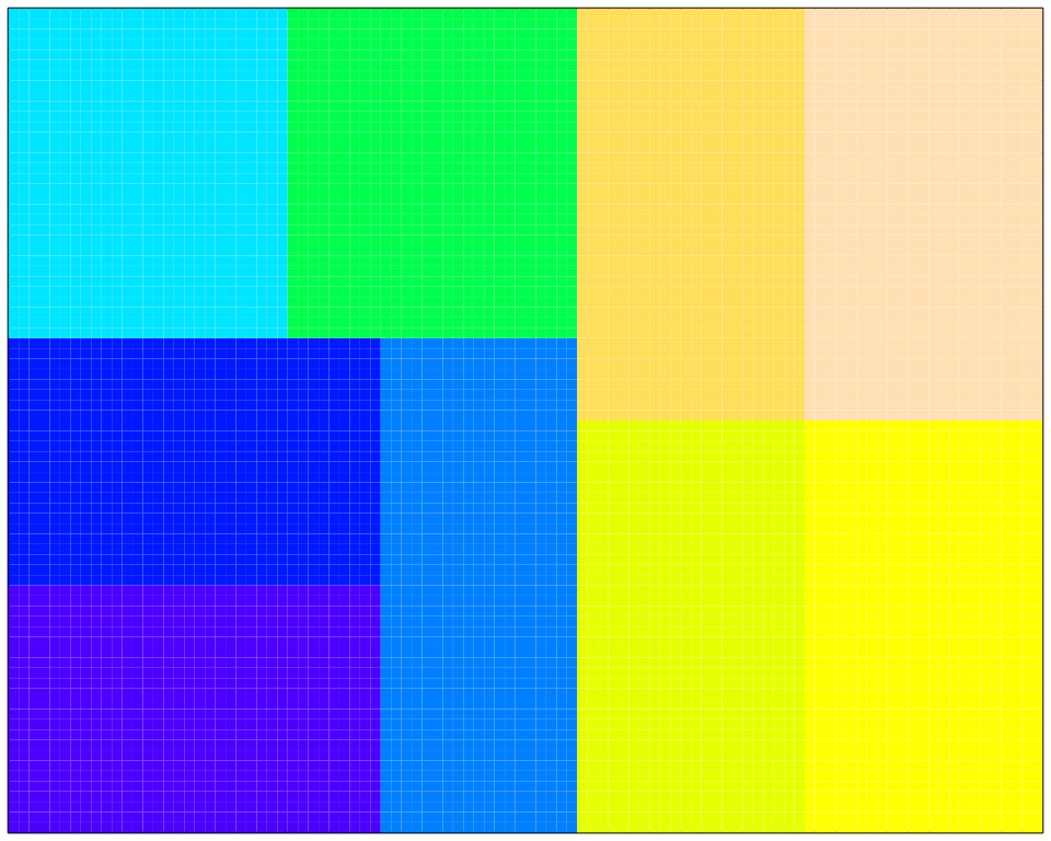
In the case of the above landscape, the number of cells allocated to each user ranges from 864 to 920.
6.2. Varying land ownership: ownership_var
In addition, whereas in previous versions variable
landscape ownership among users had to be customised using
gmse_apply, GMSE v. 0.6+ now includes an additional
parameter ownership_var, which takes effect when
land_ownership = TRUE. The value of this parameter is
expected to be >=0 and <1. At its default value of 0, land
ownership is equal among users as demonstrated in the code above. Values
>0 increase the extent of variability of landownership among users;
in technical terms, ownership_var controls the extent to
which each split in the shortest-splitline algorithm is proportional to
the number of users the landscape is to be divided into, with larger
numbers shifting the split away from even distribution. In practical
terms, this means that increasing values of ownership_var
produce more unevenly distributed landscapes among users. For example, a
value of ownership_var = 0.1 produces a relatively limited
about of inequity in landscape distribution among users.
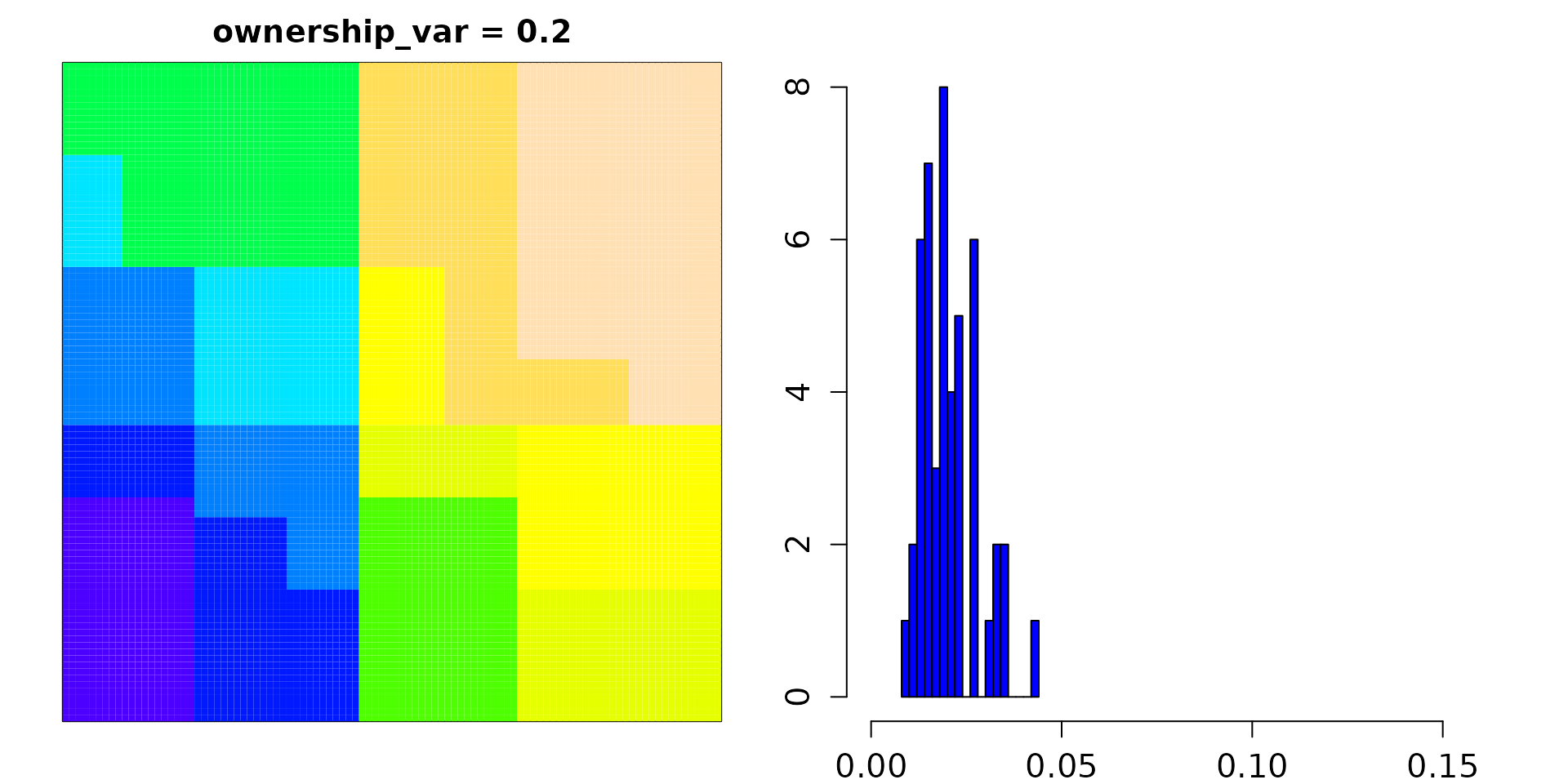 As can be seen from the frequency distribution, in this case, all users
own between 1% and 4.3% of the landscape.
As can be seen from the frequency distribution, in this case, all users
own between 1% and 4.3% of the landscape.
By contrast, when increasing ownership_var to 0.8,
overall inequity increases substantially:
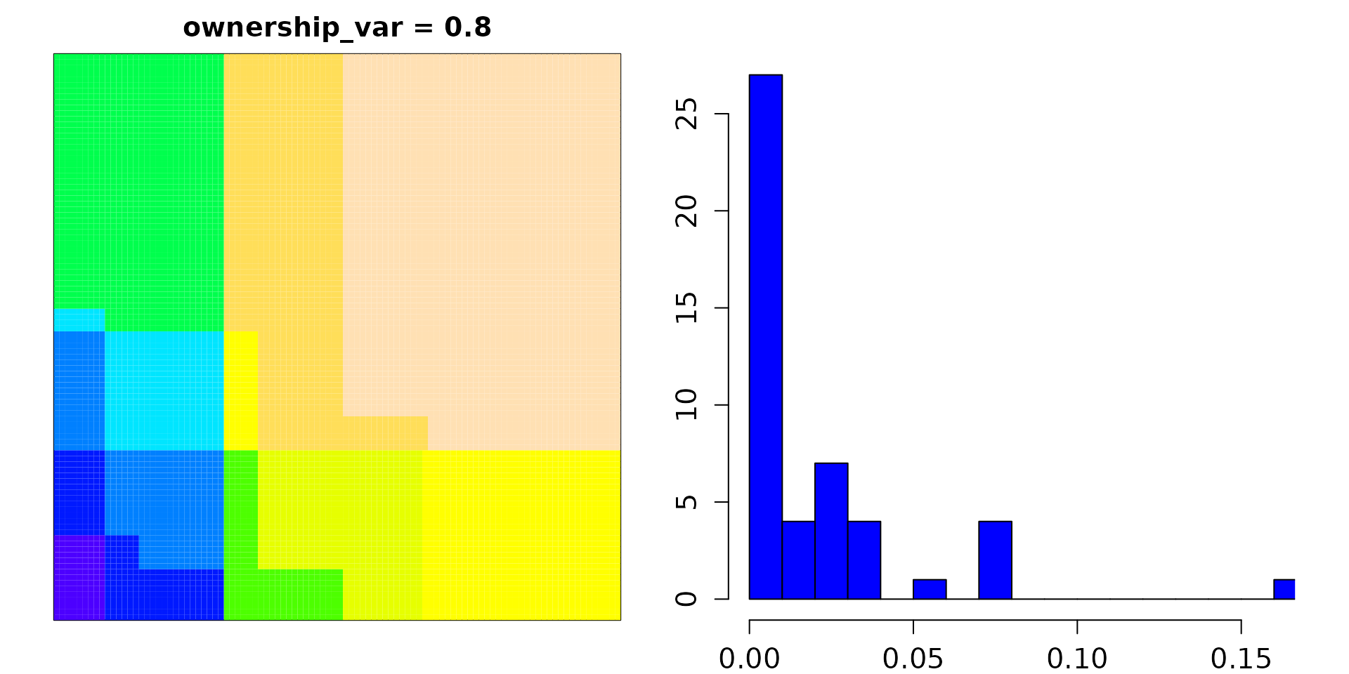
In the latter case, user ownership varies between <0.001% and 16.7%.
It should be noted that it is still entirely possible for the user to
customise landscapes to whatever extent necessary, using custom
gmse_apply loops as described
previously; however, the new ownership_var provides an
option in GMSE to alter landscape ownership in a relatively
straightforward way.
6.3. Public land
Public land is placed on the landscape whenever
public_land > 0, with public_land defining
the proportion of landscape cells that are not be owned by an user. When
the expected number of cells to be allocated to public land is
calculated to be equal to or greater than that allocated to a single
user, public land is allocated in a block as is with users. For example,
the below shows a landscape in which public_land = 0.5,
with seven other users owning land.
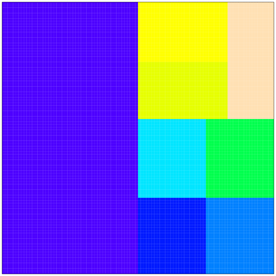
Public land is in dark blue above. If, however, the amount of public
land is very small, the land is added to the centre of the landscape.
Below illustrates a landscape that also includes seven land owning
users, but with public_land = 0.05.
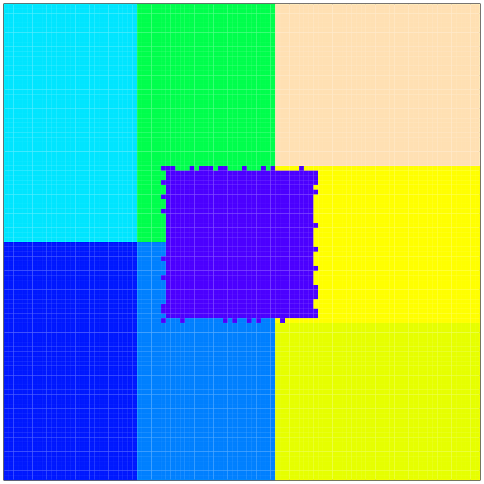
Where public_land is small, the default landscape
ownership algorithm thereby attempts to be as precise as possible in
allocating cell numbers. Of course, as previously mentioned, ownership
can also be manually specified when using gmse_apply.
Conclusions
We have focused on the data structures AGENTS, resource_array, observation_array, manager_array, user_array, and LAND because these are the data structures
that can be most readily manipulated to customise GMSE simulations. An
example of how to do this within a loop using gmse_apply
can be found in Advanced case study options.
While other data structures exist within GMSE (e.g., see the output of
gmse_apply when get_res = "Full"), we do not
recommend manipulating these structures for custom simulations.
Many data structures contain elements that are unused in GMSE v0.6+, and in all cases this is designed for ease of ongoing development of new GMSE features. Requests for new features can be made on GitHub using the GMSE Wiki or the GMSE Issues page.